Display ERP

Different ways to display a multichannel event-related potential (ERP).

# Authors: Quentin Barthélemy
#
# License: BSD (3-clause)

import numpy as np
import mne
from matplotlib import pyplot as plt
from pyriemann.utils.viz import plot_waveforms

Load EEG data

# Set filenames
data_path = str(mne.datasets.sample.data_path())
raw_fname = data_path + "/MEG/sample/sample_audvis_filt-0-40_raw.fif"
event_fname = data_path + "/MEG/sample/sample_audvis_filt-0-40_raw-eve.fif"

# Read raw data, select occipital channels and high-pass filter signal
raw = mne.io.Raw(raw_fname, preload=True, verbose=False)
raw.pick_channels(['EEG 057', 'EEG 058', 'EEG 059'], ordered=True)
raw.rename_channels({'EEG 057': 'O1', 'EEG 058': 'Oz', 'EEG 059': 'O2'})
n_channels = len(raw.ch_names)
raw.filter(1.0, None, method="iir")

# Read epochs and get responses to left visual field stimulus
tmin, tmax = -0.1, 0.8
epochs = mne.Epochs(
    raw, mne.read_events(event_fname), {'vis_l': 3}, tmin, tmax, proj=False,
    baseline=None, preload=True, verbose=False)
X = 5e5 * epochs.get_data(copy=False)
print('Number of trials:', X.shape[0])
times = np.linspace(tmin, tmax, num=X.shape[2])

plt.rcParams["figure.figsize"] = (7, 12)
ylims = []

NOTE: pick_channels() is a legacy function. New code should use inst.pick(...).
Removing projector <Projection | PCA-v1, active : False, n_channels : 102>
Removing projector <Projection | PCA-v2, active : False, n_channels : 102>
Removing projector <Projection | PCA-v3, active : False, n_channels : 102>
Filtering raw data in 1 contiguous segment
Setting up high-pass filter at 1 Hz

IIR filter parameters
---------------------
Butterworth highpass zero-phase (two-pass forward and reverse) non-causal filter:
- Filter order 8 (effective, after forward-backward)
- Cutoff at 1.00 Hz: -6.02 dB

Number of trials: 73

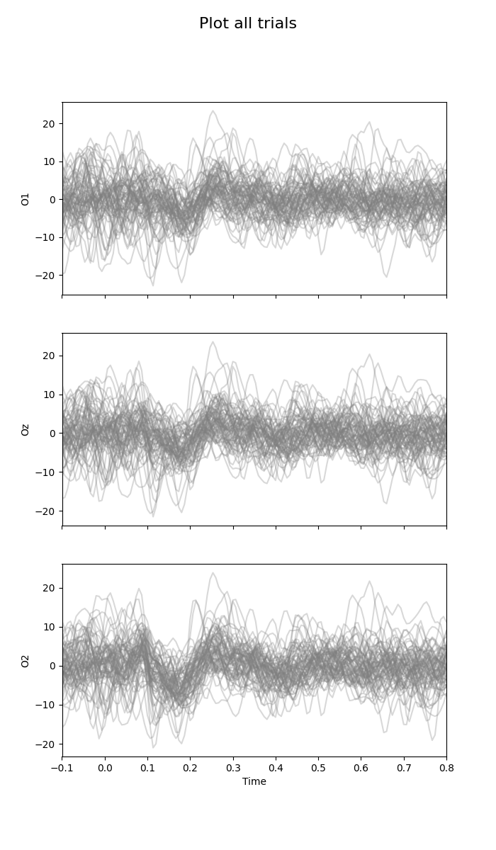
Plot all trials

This kind of plot is a little bit messy.

fig = plot_waveforms(X, 'all', times=times, alpha=0.3)
fig.suptitle('Plot all trials', fontsize=16)
for i_channel in range(n_channels):
    fig.axes[i_channel].set(ylabel=raw.ch_names[i_channel])
    fig.axes[i_channel].set_xlim(tmin, tmax)
    ylims.append(fig.axes[i_channel].get_ylim())
fig.axes[n_channels - 1].set(xlabel='Time')
plt.show()

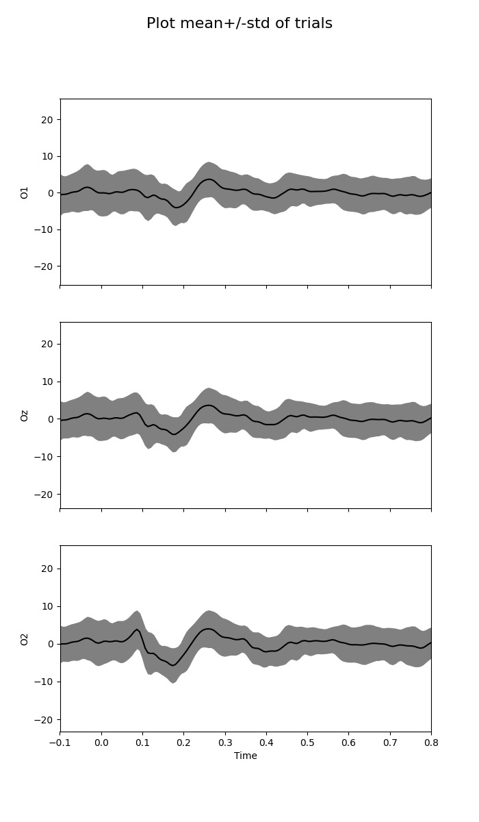
Plot central tendency and dispersion of trials

This kind of plot is well-spread, but mean and standard deviation can be contaminated by artifacts, and they make a symmetric assumption on amplitude distribution.

fig = plot_waveforms(X, 'mean+/-std', times=times)
fig.suptitle('Plot mean+/-std of trials', fontsize=16)
for i_channel in range(n_channels):
    fig.axes[i_channel].set(ylabel=raw.ch_names[i_channel])
    fig.axes[i_channel].set_xlim(tmin, tmax)
    fig.axes[i_channel].set_ylim(ylims[i_channel])
fig.axes[n_channels - 1].set(xlabel='Time')
plt.show()

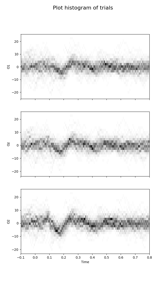
Plot histogram of trials

This plot estimates a 2D histogram of trials [1].

fig = plot_waveforms(X, 'hist', times=times, n_bins=25, cmap=plt.cm.Greys)
fig.suptitle('Plot histogram of trials', fontsize=16)
for i_channel in range(n_channels):
    fig.axes[i_channel].set(ylabel=raw.ch_names[i_channel])
    fig.axes[i_channel].set_ylim(ylims[i_channel])
fig.axes[n_channels - 1].set(xlabel='Time')
plt.show()

References

[1]

Improved estimation of EEG evoked potentials by jitter compensation and enhancing spatial filters A. Souloumiac and B. Rivet. 2013 IEEE International Conference on Acoustics, Speech and Signal Processing.