Clustering algorithm comparison

A comparison of several clustering algorithms on low-dimensional synthetic datasets, adapted to SPD matrices from [1]. The point of this example is to illustrate the nature of clustering of different algorithms, used with different metrics [2]. This should be taken with a grain of salt, as the intuition conveyed by these examples does not necessarily carry over to real datasets.

# Authors: Quentin Barthélemy
#
# License: BSD (3-clause)

from itertools import cycle, islice
from time import time

import matplotlib.pyplot as plt
import numpy as np

from pyriemann.clustering import (
    Kmeans,
    MeanShift,
)
from pyriemann.datasets import make_matrices, make_gaussian_blobs

def plot_clusterers(metric):
    fig = plt.figure(figsize=(12, 10))
    fig.suptitle(f"Clustering algorithms with metric='{metric}'", fontsize=16)
    i = 1

    # iterate over datasets
    for i_dataset, X in enumerate(datasets):
        print(f"Dataset n°{i_dataset+1}")

        x_min, x_max = X[:, 0, 0].min(), X[:, 0, 0].max()
        y_min, y_max = X[:, 0, 1].min(), X[:, 0, 1].max()
        z_min, z_max = X[:, 1, 1].min(), X[:, 1, 1].max()

        # iterate over clusterers
        for name, clt in zip(names, clusts):
            clt.set_params(**{"metric": metric})

            t0 = time()
            clt.fit(X)
            t1 = time() - t0
            if hasattr(clt, "labels_"):
                y_pred = clt.labels_.astype(int)
            else:
                y_pred = clt.predict(X)
            print(f" {name}:\n  training time={t1:.5f}")

            colors = np.array(
                list(
                    islice(
                        cycle(
                            [
                                "#377eb8",
                                "#ff7f00",
                                "#4daf4a",
                                "#f781bf",
                                "#a65628",
                                "#984ea3",
                                "#999999",
                                "#e41a1c",
                                "#dede00",
                            ]
                        ),
                        int(max(y_pred) + 1),
                    )
                )
            )
            colors = np.append(colors, ["#000000"])

            # plot
            ax = plt.subplot(n_datasets, n_clusts, i, projection="3d")
            ax.scatter(
                X[:, 0, 0],
                X[:, 0, 1],
                X[:, 1, 1],
                color=colors[y_pred]
            )

            if i_dataset == 0:
                ax.set_title(name)
            ax.set_xlim(x_min, x_max)
            ax.set_ylim(y_min, y_max)
            ax.set_zlim(z_min, z_max)
            ax.set_xticks(())
            ax.set_yticks(())
            ax.set_zticks(())
            if i_dataset <= 1:
                ax.view_init(azim=-110)
            if i_dataset == 2:
                ax.view_init(elev=20, azim=40)
            if i_dataset == 3:
                ax.view_init(elev=5, azim=100, roll=0)

            i += 1

    plt.show()

Clustering and Datasets

names = [
    "k-means, 2 clusters",
    "k-means, 3 clusters",
    "mean shift, uniform kernel",
    "mean shift, normal kernel",
]
n_jobs = 4
clusts = [
    Kmeans(n_clusters=2, n_jobs=n_jobs),
    Kmeans(n_clusters=3, n_jobs=n_jobs),
    MeanShift(kernel="uniform", n_jobs=n_jobs),
    MeanShift(kernel="normal", n_jobs=n_jobs),
]
n_clusts = len(clusts)

rs = np.random.RandomState(2025)
n_matrices, n_channels = 50, 2

datasets = [
    np.concatenate([
        make_matrices(
            n_matrices, n_channels, "spd", rs,
            evals_low=10, evals_high=14, eigvecs_mean=0.0, eigvecs_std=1.0,
        ),
        make_matrices(
            n_matrices, n_channels, "spd", rs,
            evals_low=14, evals_high=18, eigvecs_mean=5.0, eigvecs_std=2.0,
        )
    ]),
    np.concatenate([
        make_matrices(
            n_matrices, n_channels, "spd", rs,
            evals_low=4, evals_high=8, eigvecs_mean=0.0, eigvecs_std=0.5,
        ),
        make_matrices(
            n_matrices, n_channels, "spd", rs,
            evals_low=9, evals_high=13, eigvecs_mean=2.0, eigvecs_std=1.0,
        ),
        make_matrices(
            n_matrices, n_channels, "spd", rs,
            evals_low=14, evals_high=18, eigvecs_mean=5.0, eigvecs_std=2.0,
        )
    ]),
    make_gaussian_blobs(
        2*n_matrices, n_channels, random_state=rs, n_jobs=4,
        class_sep=5., class_disp=.5,
    )[0],
    make_gaussian_blobs(
        2*n_matrices, n_channels, random_state=rs, n_jobs=4,
        class_sep=2., class_disp=.5,
    )[0]
]
n_datasets = len(datasets)

Clustering with affine-invariant Riemannian metric

plot_clusterers("riemann")

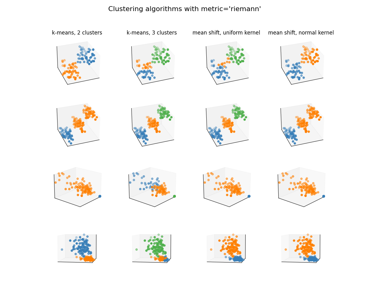
Dataset n°1
 k-means, 2 clusters:
  training time=0.21962
 k-means, 3 clusters:
  training time=0.19927
MeanShift bandwidth=0.178
 mean shift, uniform kernel:
  training time=0.58929
MeanShift bandwidth=0.178
 mean shift, normal kernel:
  training time=0.81161
Dataset n°2
 k-means, 2 clusters:
  training time=0.13636
 k-means, 3 clusters:
  training time=0.18923
MeanShift bandwidth=0.384
 mean shift, uniform kernel:
  training time=1.52271
MeanShift bandwidth=0.384
 mean shift, normal kernel:
  training time=4.89993
Dataset n°3
 k-means, 2 clusters:
  training time=0.11880
 k-means, 3 clusters:
  training time=0.41920
MeanShift bandwidth=0.837
 mean shift, uniform kernel:
  training time=2.11213
MeanShift bandwidth=0.837
 mean shift, normal kernel:
  training time=2.66837
Dataset n°4
 k-means, 2 clusters:
  training time=0.18761
 k-means, 3 clusters:
  training time=0.73375
MeanShift bandwidth=0.810
 mean shift, uniform kernel:
  training time=1.97608
MeanShift bandwidth=0.810
 mean shift, normal kernel:
  training time=2.64879

Clustering with Euclidean metric

plot_clusterers("euclid")

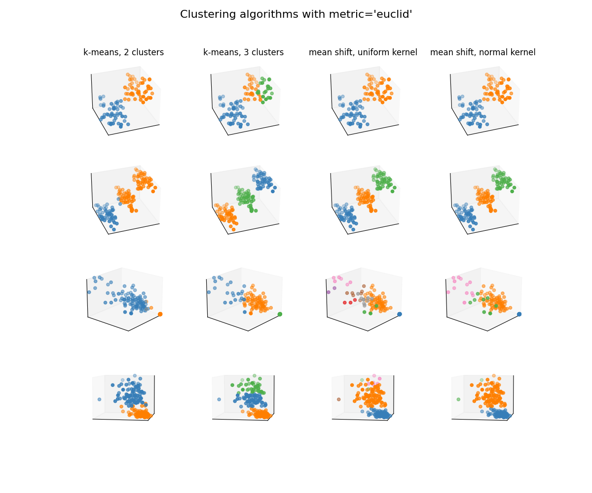
Dataset n°1
 k-means, 2 clusters:
  training time=0.03622
 k-means, 3 clusters:
  training time=0.05589
MeanShift bandwidth=2.449
 mean shift, uniform kernel:
  training time=0.20447
MeanShift bandwidth=2.449
 mean shift, normal kernel:
  training time=0.32252
Dataset n°2
 k-means, 2 clusters:
  training time=0.05578
 k-means, 3 clusters:
  training time=0.08735
MeanShift bandwidth=3.290
 mean shift, uniform kernel:
  training time=0.23260
MeanShift bandwidth=3.290
 mean shift, normal kernel:
  training time=0.41690
Dataset n°3
 k-means, 2 clusters:
  training time=0.07516
 k-means, 3 clusters:
  training time=0.19852
MeanShift bandwidth=2.257
 mean shift, uniform kernel:
  training time=0.69642
MeanShift bandwidth=2.257
 mean shift, normal kernel:
  training time=1.21742
Dataset n°4
 k-means, 2 clusters:
  training time=0.05568
 k-means, 3 clusters:
  training time=0.15730
MeanShift bandwidth=1.552
 mean shift, uniform kernel:
  training time=0.68833
MeanShift bandwidth=1.552
 mean shift, normal kernel:
  training time=1.21402

References

[1]

https://scikit-learn.org/stable/auto_examples/cluster/plot_cluster_comparison.html # noqa

[2]

Review of Riemannian distances and divergences, applied to SSVEP-based BCI S. Chevallier, E. K. Kalunga, Q. Barthélemy, E. Monacelli. Neuroinformatics, Springer, 2021, 19 (1), pp.93-106