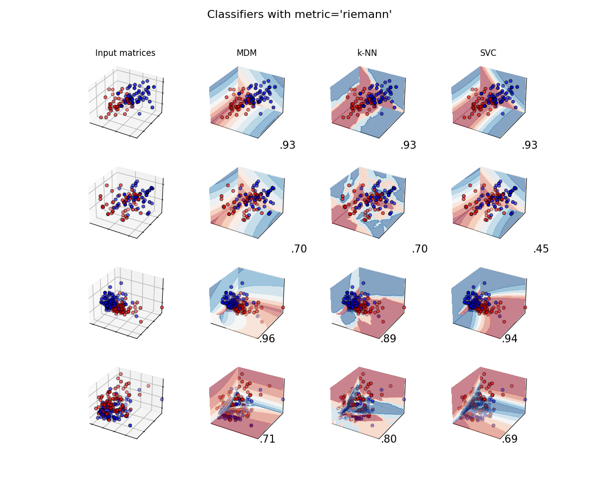
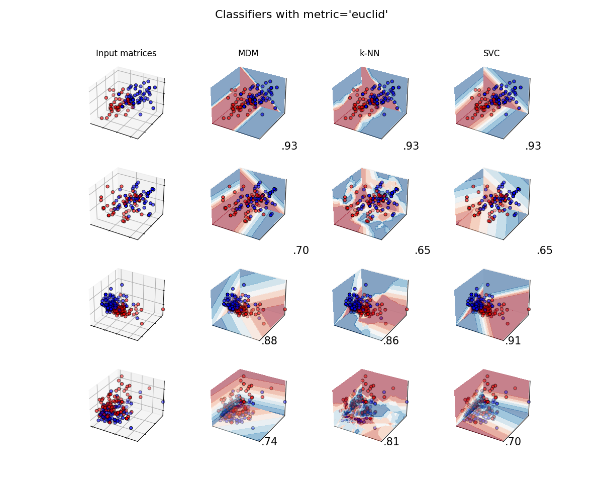
Classifier comparison

A comparison of several classifiers on low-dimensional synthetic datasets, adapted to SPD matrices from [1]. The point of this example is to illustrate the nature of decision boundaries of different classifiers, used with different metrics [2]. This should be taken with a grain of salt, as the intuition conveyed by these examples does not necessarily carry over to real datasets.

The 3D plots show training matrices in solid colors and testing matrices semi-transparent. The lower right shows the classification accuracy on the test set.

# Authors: Quentin Barthélemy
#
# License: BSD (3-clause)

from functools import partial
from time import time
import warnings

import matplotlib.pyplot as plt
from matplotlib.colors import ListedColormap
import numpy as np
from sklearn.model_selection import train_test_split

from pyriemann.classification import (
    MDM,
    KNearestNeighbor,
    SVC,
)
from pyriemann.datasets import make_matrices, make_gaussian_blobs

@partial(np.vectorize, excluded=["clf"])
def get_proba(cov_00, cov_01, cov_11, clf):
    cov = np.array([[cov_00, cov_01], [cov_01, cov_11]])
    with warnings.catch_warnings():
        warnings.simplefilter("ignore", category=RuntimeWarning)
        return clf.predict_proba(cov[np.newaxis, ...])[0, 1]


def plot_classifiers(metric):
    fig = plt.figure(figsize=(12, 10))
    fig.suptitle(f"Classifiers with metric='{metric}'", fontsize=16)
    i = 1

    # iterate over datasets
    for i_dataset, (X, y) in enumerate(datasets):
        print(f"Dataset n°{i_dataset+1}")

        # split dataset into training and test part
        X_train, X_test, y_train, y_test = train_test_split(
            X, y, test_size=0.4, random_state=42
        )

        x_min, x_max = X[:, 0, 0].min(), X[:, 0, 0].max()
        y_min, y_max = X[:, 0, 1].min(), X[:, 0, 1].max()
        z_min, z_max = X[:, 1, 1].min(), X[:, 1, 1].max()

        # just plot the dataset first
        ax = plt.subplot(n_datasets, n_classifs + 1, i, projection="3d")
        if i_dataset == 0:
            ax.set_title("Input matrices")
        # plot the training matrices
        ax.scatter(
            X_train[:, 0, 0],
            X_train[:, 0, 1],
            X_train[:, 1, 1],
            c=y_train,
            cmap=cm_bright,
            edgecolors="k"
        )
        # plot the testing matrices
        ax.scatter(
            X_test[:, 0, 0],
            X_test[:, 0, 1],
            X_test[:, 1, 1],
            c=y_test,
            cmap=cm_bright,
            alpha=0.6,
            edgecolors="k"
        )
        ax.set_xlim(x_min, x_max)
        ax.set_ylim(y_min, y_max)
        ax.set_zlim(z_min, z_max)
        ax.set_xticklabels(())
        ax.set_yticklabels(())
        ax.set_zticklabels(())
        i += 1

        rx = np.arange(x_min, x_max, (x_max - x_min) / 50)
        ry = np.arange(y_min, y_max, (y_max - y_min) / 50)
        rz = np.arange(z_min, z_max, (z_max - z_min) / 50)

        # iterate over classifiers
        for name, clf in zip(names, classifs):
            clf.set_params(**{"metric": metric})

            t0 = time()
            clf.fit(X_train, y_train)
            t1 = time() - t0
            t0 = time()
            score = clf.score(X_test, y_test)
            t2 = time() - t0
            print(
                f" {name}:\n  training time={t1:.5f}\n  test time    ={t2:.5f}"
            )

            ax = plt.subplot(n_datasets, n_classifs + 1, i, projection="3d")

            # plot the decision boundaries for horizontal 2D planes going
            # through the mean value of the third coordinates
            xx, yy = np.meshgrid(rx, ry)
            zz = get_proba(xx, yy, X[:, 1, 1].mean()*np.ones_like(xx), clf=clf)
            zz = np.ma.masked_where(~np.isfinite(zz), zz)
            ax.contourf(xx, yy, zz, zdir="z", offset=z_min, cmap=cm, alpha=0.5)

            xx, zz = np.meshgrid(rx, rz)
            yy = get_proba(xx, X[:, 0, 1].mean()*np.ones_like(xx), zz, clf=clf)
            yy = np.ma.masked_where(~np.isfinite(yy), yy)
            ax.contourf(xx, yy, zz, zdir="y", offset=y_max, cmap=cm, alpha=0.5)

            yy, zz = np.meshgrid(ry, rz)
            xx = get_proba(X[:, 0, 0].mean()*np.ones_like(yy), yy, zz, clf=clf)
            xx = np.ma.masked_where(~np.isfinite(xx), xx)
            ax.contourf(xx, yy, zz, zdir="x", offset=x_min, cmap=cm, alpha=0.5)

            # plot the training matrices
            ax.scatter(
                X_train[:, 0, 0],
                X_train[:, 0, 1],
                X_train[:, 1, 1],
                c=y_train,
                cmap=cm_bright,
                edgecolors="k"
            )
            # plot the testing matrices
            ax.scatter(
                X_test[:, 0, 0],
                X_test[:, 0, 1],
                X_test[:, 1, 1],
                c=y_test,
                cmap=cm_bright,
                edgecolors="k",
                alpha=0.6
            )

            if i_dataset == 0:
                ax.set_title(name)
            ax.text(
                1.3 * x_max,
                y_min,
                z_min,
                ("%.2f" % score).lstrip("0"),
                size=15,
                horizontalalignment="right",
                verticalalignment="bottom"
            )
            ax.set_xlim(x_min, x_max)
            ax.set_ylim(y_min, y_max)
            ax.set_zlim(z_min, z_max)
            ax.set_xticks(())
            ax.set_yticks(())
            ax.set_zticks(())

            i += 1

    plt.show()

Classifiers and Datasets

names = [
    "MDM",
    "k-NN",
    "SVC",
]
classifs = [
    MDM(),
    KNearestNeighbor(n_neighbors=3),
    SVC(probability=True),
]
n_classifs = len(classifs)

rs = np.random.RandomState(2022)
n_matrices, n_channels = 50, 2
y = np.concatenate([np.zeros(n_matrices), np.ones(n_matrices)])

datasets = [
    (
        np.concatenate([
            make_matrices(
                n_matrices, n_channels, "spd", rs, evals_low=10, evals_high=14
            ),
            make_matrices(
                n_matrices, n_channels, "spd", rs, evals_low=13, evals_high=17
            )
        ]),
        y
    ),
    (
        np.concatenate([
            make_matrices(
                n_matrices, n_channels, "spd", rs, evals_low=10, evals_high=14
            ),
            make_matrices(
                n_matrices, n_channels, "spd", rs, evals_low=11, evals_high=15
            )
        ]),
        y
    ),
    make_gaussian_blobs(
        2*n_matrices, n_channels, random_state=rs, class_sep=1., class_disp=.5,
        n_jobs=4
    ),
    make_gaussian_blobs(
        2*n_matrices, n_channels, random_state=rs, class_sep=.5, class_disp=.5,
        n_jobs=4
    )
]
n_datasets = len(datasets)

cm = plt.cm.RdBu
cm_bright = ListedColormap(["#FF0000", "#0000FF"])

Classifiers with affine-invariant Riemannian metric

plot_classifiers("riemann")

Dataset n°1
 MDM:
  training time=0.00225
  test time    =0.00106
 k-NN:
  training time=0.00004
  test time    =0.00841
 SVC:
  training time=0.00253
  test time    =0.00093
Dataset n°2
 MDM:
  training time=0.00221
  test time    =0.00098
 k-NN:
  training time=0.00003
  test time    =0.00834
 SVC:
  training time=0.00252
  test time    =0.00094
Dataset n°3
 MDM:
  training time=0.00363
  test time    =0.00099
 k-NN:
  training time=0.00006
  test time    =0.01877
 SVC:
  training time=0.00423
  test time    =0.00112
Dataset n°4
 MDM:
  training time=0.00412
  test time    =0.00100
 k-NN:
  training time=0.00004
  test time    =0.01886
 SVC:
  training time=0.00413
  test time    =0.00110

Classifiers with Euclidean metric

plot_classifiers("euclid")

Dataset n°1
 MDM:
  training time=0.00040
  test time    =0.00073
 k-NN:
  training time=0.00003
  test time    =0.00278
 SVC:
  training time=0.00088
  test time    =0.00063
Dataset n°2
 MDM:
  training time=0.00035
  test time    =0.00074
 k-NN:
  training time=0.00003
  test time    =0.00283
 SVC:
  training time=0.00113
  test time    =0.00065
Dataset n°3
 MDM:
  training time=0.00035
  test time    =0.00070
 k-NN:
  training time=0.00003
  test time    =0.00477
 SVC:
  training time=0.00112
  test time    =0.00063
Dataset n°4
 MDM:
  training time=0.00038
  test time    =0.00068
 k-NN:
  training time=0.00003
  test time    =0.00484
 SVC:
  training time=0.00157
  test time    =0.00064

References

[1]

https://scikit-learn.org/stable/auto_examples/classification/plot_classifier_comparison.html # noqa

[2]

Review of Riemannian distances and divergences, applied to SSVEP-based BCI S. Chevallier, E. K. Kalunga, Q. Barthélemy, E. Monacelli. Neuroinformatics, Springer, 2021, 19 (1), pp.93-106