Note
Go to the end to download the full example code.
Classifier comparison
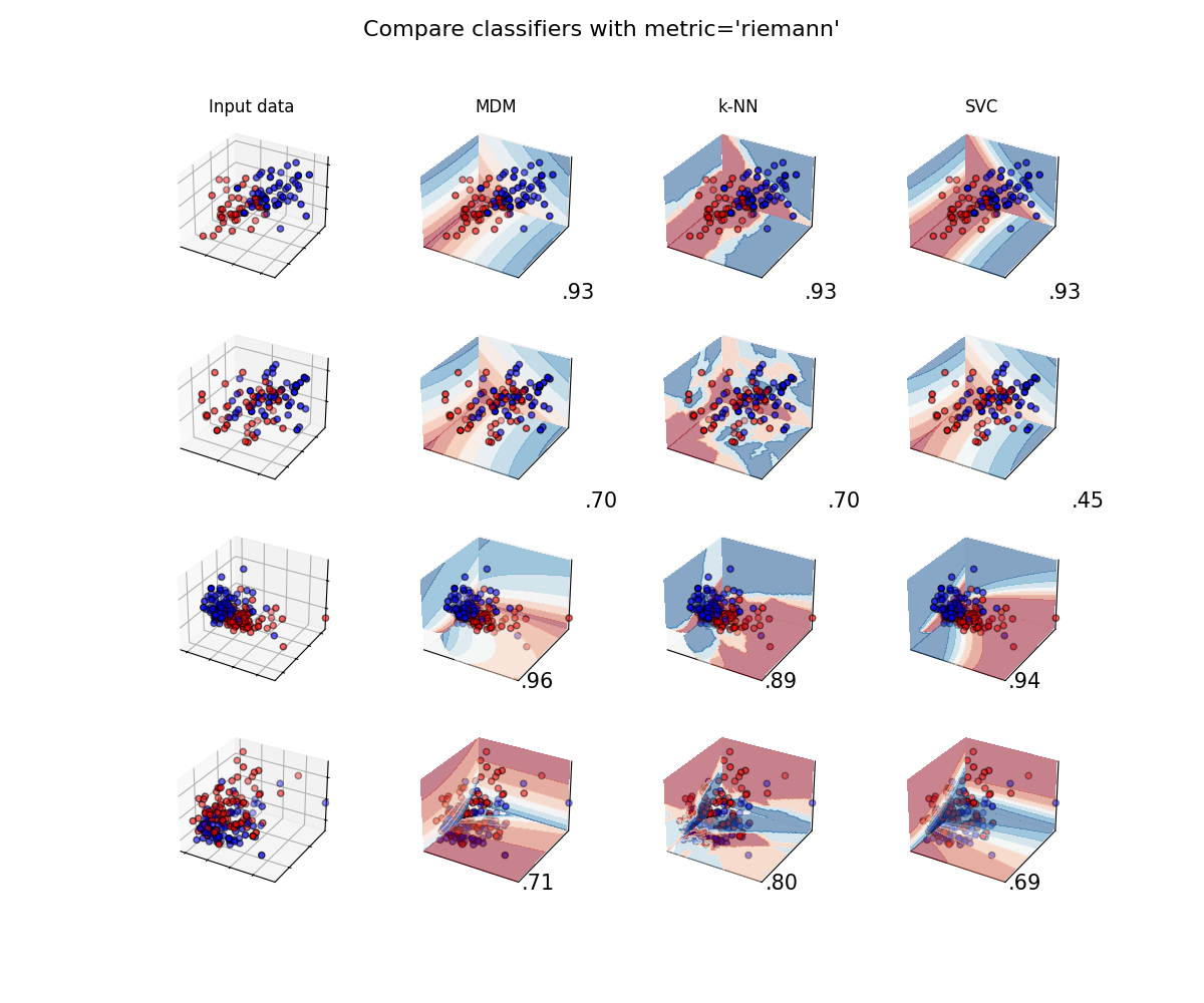
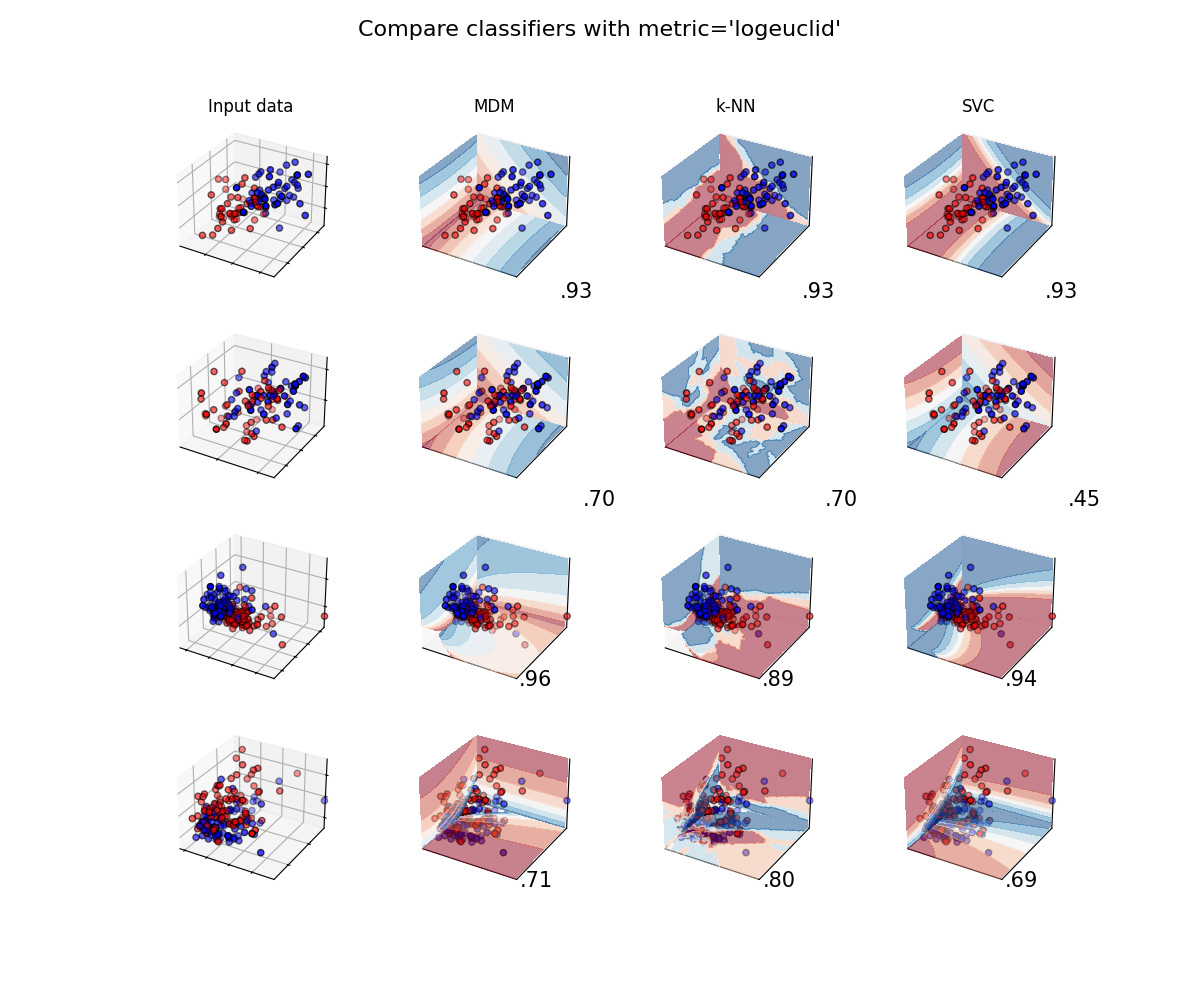
A comparison of several classifiers on low-dimensional synthetic datasets, adapted to SPD matrices from [1]. The point of this example is to illustrate the nature of decision boundaries of different classifiers, used with different metrics [2]. This should be taken with a grain of salt, as the intuition conveyed by these examples does not necessarily carry over to real datasets.
The 3D plots show training matrices in solid colors and testing matrices semi-transparent. The lower right shows the classification accuracy on the test set.
# Authors: Quentin Barthélemy
#
# License: BSD (3-clause)

from functools import partial
from time import time

import matplotlib.pyplot as plt
from matplotlib.colors import ListedColormap
import numpy as np
from sklearn.model_selection import train_test_split

from pyriemann.classification import (
    MDM,
    KNearestNeighbor,
    SVC,
)
from pyriemann.datasets import make_matrices, make_gaussian_blobs
@partial(np.vectorize, excluded=["clf"])
def get_proba(cov_00, cov_01, cov_11, clf):
    cov = np.array([[cov_00, cov_01], [cov_01, cov_11]])
    with np.testing.suppress_warnings() as sup:
        sup.filter(RuntimeWarning)
        return clf.predict_proba(cov[np.newaxis, ...])[0, 1]


def plot_classifiers(metric):
    figure = plt.figure(figsize=(12, 10))
    figure.suptitle(f"Compare classifiers with metric='{metric}'", fontsize=16)
    i = 1

    # iterate over datasets
    for ds_cnt, (X, y) in enumerate(datasets):
        # split dataset into training and test part
        X_train, X_test, y_train, y_test = train_test_split(
            X, y, test_size=0.4, random_state=42
        )

        x_min, x_max = X[:, 0, 0].min(), X[:, 0, 0].max()
        y_min, y_max = X[:, 0, 1].min(), X[:, 0, 1].max()
        z_min, z_max = X[:, 1, 1].min(), X[:, 1, 1].max()

        # just plot the dataset first
        ax = plt.subplot(n_datasets, n_classifs + 1, i, projection="3d")
        if ds_cnt == 0:
            ax.set_title("Input data")
        # Plot the training points
        ax.scatter(
            X_train[:, 0, 0],
            X_train[:, 0, 1],
            X_train[:, 1, 1],
            c=y_train,
            cmap=cm_bright,
            edgecolors="k"
        )
        # Plot the testing points
        ax.scatter(
            X_test[:, 0, 0],
            X_test[:, 0, 1],
            X_test[:, 1, 1],
            c=y_test,
            cmap=cm_bright,
            alpha=0.6,
            edgecolors="k"
        )
        ax.set_xlim(x_min, x_max)
        ax.set_ylim(y_min, y_max)
        ax.set_zlim(z_min, z_max)
        ax.set_xticklabels(())
        ax.set_yticklabels(())
        ax.set_zticklabels(())
        i += 1

        rx = np.arange(x_min, x_max, (x_max - x_min) / 50)
        ry = np.arange(y_min, y_max, (y_max - y_min) / 50)
        rz = np.arange(z_min, z_max, (z_max - z_min) / 50)

        print(f"Dataset n°{ds_cnt+1}")

        # iterate over classifiers
        for name, clf in zip(names, classifiers):
            ax = plt.subplot(n_datasets, n_classifs + 1, i, projection="3d")

            clf.set_params(**{"metric": metric})
            t0 = time()
            clf.fit(X_train, y_train)
            t1 = time() - t0

            t0 = time()
            score = clf.score(X_test, y_test)
            t2 = time() - t0

            print(
                f" {name}:\n  training time={t1:.5f}\n  test time    ={t2:.5f}"
            )

            # Plot the decision boundaries for horizontal 2D planes going
            # through the mean value of the third coordinates
            xx, yy = np.meshgrid(rx, ry)
            zz = get_proba(xx, yy, X[:, 1, 1].mean()*np.ones_like(xx), clf=clf)
            zz = np.ma.masked_where(~np.isfinite(zz), zz)
            ax.contourf(xx, yy, zz, zdir="z", offset=z_min, cmap=cm, alpha=0.5)

            xx, zz = np.meshgrid(rx, rz)
            yy = get_proba(xx, X[:, 0, 1].mean()*np.ones_like(xx), zz, clf=clf)
            yy = np.ma.masked_where(~np.isfinite(yy), yy)
            ax.contourf(xx, yy, zz, zdir="y", offset=y_max, cmap=cm, alpha=0.5)

            yy, zz = np.meshgrid(ry, rz)
            xx = get_proba(X[:, 0, 0].mean()*np.ones_like(yy), yy, zz, clf=clf)
            xx = np.ma.masked_where(~np.isfinite(xx), xx)
            ax.contourf(xx, yy, zz, zdir="x", offset=x_min, cmap=cm, alpha=0.5)

            # Plot the training points
            ax.scatter(
                X_train[:, 0, 0],
                X_train[:, 0, 1],
                X_train[:, 1, 1],
                c=y_train,
                cmap=cm_bright,
                edgecolors="k"
            )
            # Plot the testing points
            ax.scatter(
                X_test[:, 0, 0],
                X_test[:, 0, 1],
                X_test[:, 1, 1],
                c=y_test,
                cmap=cm_bright,
                edgecolors="k",
                alpha=0.6
            )

            if ds_cnt == 0:
                ax.set_title(name)
            ax.text(
                1.3 * x_max,
                y_min,
                z_min,
                ("%.2f" % score).lstrip("0"),
                size=15,
                horizontalalignment="right",
                verticalalignment="bottom"
            )
            ax.set_xlim(x_min, x_max)
            ax.set_ylim(y_min, y_max)
            ax.set_zlim(z_min, z_max)
            ax.set_xticks(())
            ax.set_yticks(())
            ax.set_zticks(())

            i += 1

    plt.show()
Classifiers and Datasets
names = [
    "MDM",
    "k-NN",
    "SVC",
]
classifiers = [
    MDM(),
    KNearestNeighbor(n_neighbors=3),
    SVC(probability=True),
]
n_classifs = len(classifiers)

rs = np.random.RandomState(2022)
n_matrices, n_channels = 50, 2
y = np.concatenate([np.zeros(n_matrices), np.ones(n_matrices)])

datasets = [
    (
        np.concatenate([
            make_matrices(
                n_matrices, n_channels, "spd", rs, evals_low=10, evals_high=14
            ),
            make_matrices(
                n_matrices, n_channels, "spd", rs, evals_low=13, evals_high=17
            )
        ]),
        y
    ),
    (
        np.concatenate([
            make_matrices(
                n_matrices, n_channels, "spd", rs, evals_low=10, evals_high=14
            ),
            make_matrices(
                n_matrices, n_channels, "spd", rs, evals_low=11, evals_high=15
            )
        ]),
        y
    ),
    make_gaussian_blobs(
        2*n_matrices, n_channels, random_state=rs, class_sep=1., class_disp=.5,
        n_jobs=4
    ),
    make_gaussian_blobs(
        2*n_matrices, n_channels, random_state=rs, class_sep=.5, class_disp=.5,
        n_jobs=4
    )
]
n_datasets = len(datasets)

cm = plt.cm.RdBu
cm_bright = ListedColormap(["#FF0000", "#0000FF"])
Classifiers with Riemannian metric
plot_classifiers("riemann")
Dataset n°1
 MDM:
  training time=0.00124
  test time    =0.00278
 k-NN:
  training time=0.00005
  test time    =0.05967
 SVC:
  training time=0.00219
  test time    =0.00100
Dataset n°2
 MDM:
  training time=0.00137
  test time    =0.00257
 k-NN:
  training time=0.00003
  test time    =0.06048
 SVC:
  training time=0.00245
  test time    =0.00108
Dataset n°3
 MDM:
  training time=0.00229
  test time    =0.00457
 k-NN:
  training time=0.00003
  test time    =0.23168
 SVC:
  training time=0.00340
  test time    =0.00111
Dataset n°4
 MDM:
  training time=0.00266
  test time    =0.00466
 k-NN:
  training time=0.00003
  test time    =0.23179
 SVC:
  training time=0.00343
  test time    =0.00113
Classifiers with Log-Euclidean metric
plot_classifiers("logeuclid")
Dataset n°1
 MDM:
  training time=0.00047
  test time    =0.00430
 k-NN:
  training time=0.00004
  test time    =0.10280
 SVC:
  training time=0.00141
  test time    =0.00100
Dataset n°2
 MDM:
  training time=0.00038
  test time    =0.00397
 k-NN:
  training time=0.00003
  test time    =0.10297
 SVC:
  training time=0.00148
  test time    =0.00098
Dataset n°3
 MDM:
  training time=0.00045
  test time    =0.00748
 k-NN:
  training time=0.00004
  test time    =0.40898
 SVC:
  training time=0.00179
  test time    =0.00121
Dataset n°4
 MDM:
  training time=0.00053
  test time    =0.00741
 k-NN:
  training time=0.00003
  test time    =0.40293
 SVC:
  training time=0.00189
  test time    =0.00112
Classifiers with Euclidean metric
plot_classifiers("euclid")

Dataset n°1
 MDM:
  training time=0.00021
  test time    =0.00101
 k-NN:
  training time=0.00004
  test time    =0.01392
 SVC:
  training time=0.00096
  test time    =0.00082
Dataset n°2
 MDM:
  training time=0.00020
  test time    =0.00096
 k-NN:
  training time=0.00004
  test time    =0.01419
 SVC:
  training time=0.00127
  test time    =0.00075
Dataset n°3
 MDM:
  training time=0.00019
  test time    =0.00142
 k-NN:
  training time=0.00003
  test time    =0.05170
 SVC:
  training time=0.00130
  test time    =0.00077
Dataset n°4
 MDM:
  training time=0.00020
  test time    =0.00140
 k-NN:
  training time=0.00003
  test time    =0.05270
 SVC:
  training time=0.00177
  test time    =0.00082
References
Total running time of the script: (4 minutes 29.702 seconds)