Visualization of SSVEP-based BCI Classification in Tangent Space

Project extended covariance matrices of SSVEP-based BCI in the tangent space, using principal geodesic analysis (PGA).

You should have a look to “Offline SSVEP-based BCI Multiclass Prediction” before this example.

# Authors: Quentin Barthélemy, Emmanuel Kalunga and Sylvain Chevallier
#
# License: BSD (3-clause)

import numpy as np
import matplotlib.pyplot as plt
from matplotlib.animation import FuncAnimation
from mne import find_events, Epochs, make_fixed_length_epochs
from mne.io import Raw
from sklearn.pipeline import make_pipeline
from sklearn.decomposition import PCA

from pyriemann.estimation import BlockCovariances
from pyriemann.classification import MDM
from pyriemann.tangentspace import TangentSpace
from pyriemann.utils.viz import _add_alpha
from helpers.ssvep_helpers import download_data, extend_signal

clabel = ['resting-state', '13 Hz', '17 Hz', '21 Hz']
clist = plt.cm.viridis(np.array([0, 1, 2, 3])/3)
cmap = "viridis"


def plot_pga(ax, data, labels, centers):
    sc = ax.scatter(data[:, 0], data[:, 1], c=labels, marker='P', cmap=cmap)
    ax.scatter(
        centers[:, 0], centers[:, 1], c=clist, marker='o', s=100, cmap=cmap
        )
    ax.set(xlabel='PGA, 1st axis', ylabel='PGA, 2nd axis')
    for i in range(len(clabel)):
        ax.scatter([], [], color=clist[i], marker='o', s=50, label=clabel[i])
    ax.legend(loc='upper right')
    return sc

Load EEG and extract covariance matrices for SSVEP

frequencies = [13, 17, 21]
freq_band = 0.1
events_id = {'13 Hz': 2, '17 Hz': 4, '21 Hz': 3, 'resting-state': 1}

duration = 2.5    # duration of epochs
interval = 0.25   # interval between successive epochs for online processing

# Subject 12: first 4 sessions for training, last session for test

# Training set
raw = Raw(download_data(subject=12, session=1), preload=True, verbose=False)
events = find_events(raw, shortest_event=0, verbose=False)
raw = raw.pick("eeg")
ch_count = len(raw.info['ch_names'])
raw_ext = extend_signal(raw, frequencies, freq_band)
epochs = Epochs(
    raw_ext, events, events_id, tmin=2, tmax=5, baseline=None, verbose=False
).get_data(copy=False)
x_train = BlockCovariances(
    estimator='lwf', block_size=ch_count
).transform(epochs)
y_train = events[:, 2]

# Testing set
raw = Raw(download_data(subject=12, session=4), preload=True, verbose=False)
raw = raw.pick_types(eeg=True)
raw_ext = extend_signal(raw, frequencies, freq_band)
epochs = make_fixed_length_epochs(
    raw_ext, duration=duration, overlap=duration - interval, verbose=False
).get_data(copy=False)
x_test = BlockCovariances(
    estimator='lwf', block_size=ch_count
).transform(epochs)

Download complete in 00s (3.2 MB)
Creating RawArray with float64 data, n_channels=24, n_times=92384
    Range : 0 ... 92383 =      0.000 ...   360.871 secs
Ready.
Using data from preloaded Raw for 32 events and 769 original time points ...
0 bad epochs dropped

  0%|                                              | 0.00/5.35M [00:00<?, ?B/s]
  0%|                                      | 14.3k/5.35M [00:00<00:46, 115kB/s]
  1%|▎                                     | 41.0k/5.35M [00:00<00:27, 192kB/s]
  2%|▊                                      | 106k/5.35M [00:00<00:13, 384kB/s]
  4%|█▋                                     | 233k/5.35M [00:00<00:07, 708kB/s]
  9%|███▎                                  | 459k/5.35M [00:00<00:03, 1.23MB/s]
 17%|██████▌                               | 916k/5.35M [00:00<00:01, 2.30MB/s]
 35%|████████████▉                        | 1.88M/5.35M [00:00<00:00, 4.56MB/s]
 64%|███████████████████████▊             | 3.45M/5.35M [00:00<00:00, 7.92MB/s]
 93%|██████████████████████████████████▌  | 5.00M/5.35M [00:00<00:00, 10.1MB/s]
  0%|                                              | 0.00/5.35M [00:00<?, ?B/s]
100%|█████████████████████████████████████| 5.35M/5.35M [00:00<00:00, 21.5GB/s]
Download complete in 01s (5.1 MB)
NOTE: pick_types() is a legacy function. New code should use inst.pick(...).
Creating RawArray with float64 data, n_channels=24, n_times=148544
    Range : 0 ... 148543 =      0.000 ...   580.246 secs
Ready.
Using data from preloaded Raw for 2312 events and 640 original time points ...
0 bad epochs dropped

Classification with minimum distance to mean (MDM)

Classification for a 4-class SSVEP BCI, including resting-state class.

print("Number of training trials: {}".format(len(x_train)))

mdm = MDM(metric=dict(mean='riemann', distance='riemann'))
mdm.fit(x_train, y_train)

Number of training trials: 32

MDM(metric={'distance': 'riemann', 'mean': 'riemann'})

In a Jupyter environment, please rerun this cell to show the HTML representation or trust the notebook.
On GitHub, the HTML representation is unable to render, please try loading this page with nbviewer.org.

Projection in tangent space with principal geodesic analysis (PGA)

Project covariance matrices from the Riemannian manifold into the Euclidean tangent space at the grand average, and apply a principal component analysis (PCA) to obtain an unsupervised dimension reduction [1].

pga = make_pipeline(
    TangentSpace(metric="riemann", tsupdate=False),
    PCA(n_components=2)
)

ts_train = pga.fit_transform(x_train)
ts_means = pga.transform(np.array(mdm.covmeans_))

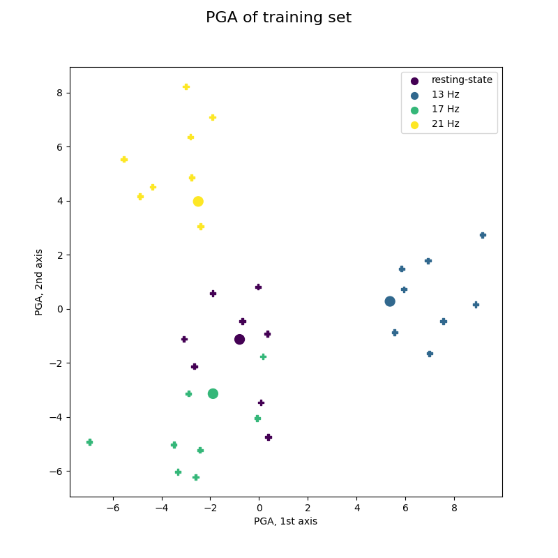
Offline training of MDM visualized by PGA

These figures show the trajectory on the tangent space taken by covariance matrices during a 4-class SSVEP experiment, and how they are classified epoch by epoch.

This figure reproduces Fig 3(c) of reference [2], showing training trials of best subject.

fig, ax = plt.subplots(figsize=(8, 8))
fig.suptitle('PGA of training set', fontsize=16)
plot_pga(ax, ts_train, y_train, ts_means)
plt.show()

/home/docs/checkouts/readthedocs.org/user_builds/pyriemann/checkouts/latest/examples/SSVEP/plot_classify_ssvep_pga.py:40: UserWarning: No data for colormapping provided via 'c'. Parameters 'cmap' will be ignored
  ax.scatter(

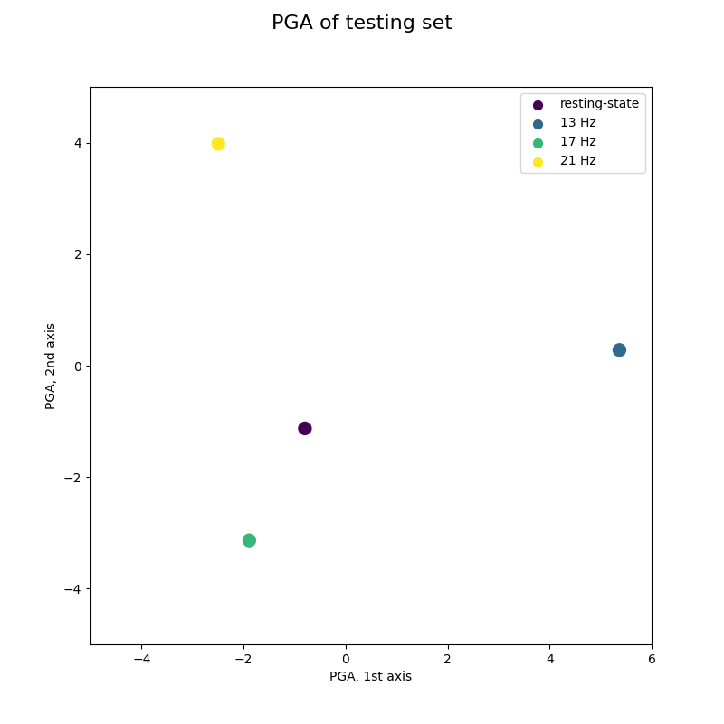
Online classification by MDM visualized by PGA

This figure reproduces Fig 6 of reference [2], with an animation to imitate an online acquisition, processing and classification of EEG time-series.

Warning: [2] uses a curved based online classification, while a single trial classification is used here.

# Prepare data for online classification
test_visu = 50     # nb of matrices to display simultaneously
colors, ts_visu = [], np.empty([0, 2])
alphas = np.linspace(0, 1, test_visu)

fig, ax = plt.subplots(figsize=(8, 8))
fig.suptitle('PGA of testing set', fontsize=16)
pl = plot_pga(ax, ts_visu, colors, ts_means)
pl.axes.set_xlim(-5, 6)
pl.axes.set_ylim(-5, 5)

(-5.0, 5.0)

# Prepare animation for online classification
def online_classify(t):
    global colors, ts_visu

    # Online classification
    y = mdm.predict(x_test[np.newaxis, t])
    color = clist[int(y[0] - 1)]
    ts_test = pga.transform(x_test[np.newaxis, t])

    # Update data
    colors.append(color)
    ts_visu = np.vstack((ts_visu, ts_test))
    if len(ts_visu) > test_visu:
        colors.pop(0)
        ts_visu = ts_visu[1:]
    colors = _add_alpha(colors, alphas)

    # Update plot
    pl.set_offsets(np.c_[ts_visu[:, 0], ts_visu[:, 1]])
    pl.set_color(colors)
    return pl


interval_display = 1.0  # can be changed for a slower display

visu = FuncAnimation(fig, online_classify,
                     frames=range(0, len(x_test)),
                     interval=interval_display, blit=False, repeat=False)

# Plot online classification

# Plot complete visu: a dynamic display is required
plt.show()

# Plot only 10s, for animated documentation
try:
    from IPython.display import HTML
except ImportError:
    raise ImportError("Install IPython to plot animation in documentation")

plt.rcParams["animation.embed_limit"] = 10
HTML(visu.to_jshtml(fps=5, default_mode='loop'))

Animation size has reached 10525072 bytes, exceeding the limit of 10485760.0. If you're sure you want a larger animation embedded, set the animation.embed_limit rc parameter to a larger value (in MB). This and further frames will be dropped.

Once Loop Reflect

References

[1]

Principal geodesic analysis for the study of nonlinear statistics of shape P.T. Fletcher, C. Lu, S. M. Pizer, S. Joshi. IEEE Transactions on Medical Imaging (Volume: 23, Issue: 8, August 2004).

[2] (1,2,3)

Online SSVEP-based BCI using Riemannian geometry E. K. Kalunga, S. Chevallier, Q. Barthélemy, K. Djouani, E. Monacelli, Y. Hamam. Neurocomputing, Elsevier, 2016, 191, pp.55-68.