Frequency band selection on the manifold for motor imagery classification

Find optimal frequency band using class distinctiveness measure on the manifold and compare classification performance for motor imagery data to the baseline with no frequency band selection [1].

# Authors: Maria Sayu Yamamoto <maria-sayu.yamamoto@universite-paris-saclay.fr>
#
# License: BSD (3-clause)

from time import time

import numpy as np
from matplotlib import pyplot as plt
from mne import Epochs, pick_types, events_from_annotations
from mne.io import concatenate_raws
from mne.io.edf import read_raw_edf
from mne.datasets import eegbci
from sklearn.model_selection import cross_val_score, ShuffleSplit

from pyriemann.classification import MDM
from pyriemann.estimation import Covariances
from helpers.frequencybandselection_helpers import freq_selection_class_dis

Set basic parameters and read data

tmin, tmax = 0.5, 2.5
event_id = dict(T1=2, T2=3)
subject = 1
runs = [4, 8, 12]  # motor imagery: left hand vs right hand

raw_files = [
    read_raw_edf(f, preload=True) for f in eegbci.load_data(subject, runs)
]
raw = concatenate_raws(raw_files)
picks = pick_types(
    raw.info, meg=False, eeg=True, stim=False, eog=False, exclude='bads')
# subsample elecs
picks = picks[::2]

# cross validation
cv = ShuffleSplit(n_splits=1, test_size=0.2, random_state=42)

Downloading EEGBCI data
Download complete in 08s (7.4 MB)
Extracting EDF parameters from /home/docs/mne_data/MNE-eegbci-data/files/eegmmidb/1.0.0/S001/S001R04.edf...
EDF file detected
Setting channel info structure...
Creating raw.info structure...
Reading 0 ... 19999  =      0.000 ...   124.994 secs...
Extracting EDF parameters from /home/docs/mne_data/MNE-eegbci-data/files/eegmmidb/1.0.0/S001/S001R08.edf...
EDF file detected
Setting channel info structure...
Creating raw.info structure...
Reading 0 ... 19999  =      0.000 ...   124.994 secs...
Extracting EDF parameters from /home/docs/mne_data/MNE-eegbci-data/files/eegmmidb/1.0.0/S001/S001R12.edf...
EDF file detected
Setting channel info structure...
Creating raw.info structure...
Reading 0 ... 19999  =      0.000 ...   124.994 secs...

Baseline pipeline without frequency band selection

Apply band-pass filter using a wide frequency band, 5-35 Hz. Train and evaluate classifier.

t0 = time()
raw_filter = raw.copy().filter(5., 35., method='iir', picks=picks,
                               verbose=False)

events, _ = events_from_annotations(raw_filter, event_id,
                                    verbose=False)

# Read epochs (train will be done only between 0.5 and 2.5 s)
epochs = Epochs(
    raw_filter,
    events,
    event_id,
    tmin,
    tmax,
    proj=True,
    picks=picks,
    baseline=None,
    preload=True,
    verbose=False)
labels = epochs.events[:, -1] - 2

# Get epochs
epochs_data_baseline = epochs.get_data(units="uV", copy=False)

# Compute covariance matrices
cov_data_baseline = Covariances().transform(epochs_data_baseline)

# Set classifier
model = MDM(metric=dict(mean='riemann', distance='riemann'))

# Classification with minimum distance to mean
acc_baseline = cross_val_score(model, cov_data_baseline, labels,
                               cv=cv, n_jobs=1)
t1 = time() - t0

Pipeline with a frequency band selection based on the class distinctiveness

Step1: Select frequency band maximizing class distinctiveness on training set.

Define parameters for frequency band selection

t2 = time()
freq_band = [5., 35.]
sub_band_width = 4.
sub_band_step = 2.
alpha = 0.4

# Select frequency band using training set
best_freq, all_class_dis = \
    freq_selection_class_dis(raw, freq_band, sub_band_width,
                             sub_band_step, alpha,
                             tmin, tmax,
                             picks, event_id,
                             cv,
                             return_class_dis=True, verbose=False)

print(f'Selected frequency band : {best_freq[0][0]} - {best_freq[0][1]} Hz')

Selected frequency band : 9.0 - 15.0 Hz

Step2: Train classifier using selected frequency band and evaluate performance using test set

# Apply band-pass filter using the best frequency band
best_raw_filter = raw.copy().filter(best_freq[0][0], best_freq[0][1],
                                    method='iir', picks=picks,
                                    verbose=False)

events, _ = events_from_annotations(best_raw_filter, event_id, verbose=False)

# Read epochs (train will be done only between 0.5 and 2.5s)
epochs = Epochs(
    best_raw_filter,
    events,
    event_id,
    tmin,
    tmax,
    proj=True,
    picks=picks,
    baseline=None,
    preload=True,
    verbose=False)

# Get epochs
epochs_data_train = epochs.get_data(units="uV", copy=False)

# Estimate covariance matrices
cov_data = Covariances().transform(epochs_data_train)

# Classification with minimum distance to mean
acc = cross_val_score(model, cov_data, labels, cv=cv, n_jobs=1)
t3 = time() - t2

Compare pipelines: accuracies and training times

print("Classification accuracy without frequency band selection: "
      + f"{acc_baseline[0]:.02f}")
print("Total computational time without frequency band selection: "
      + f"{t1:.5f} s")
print("Classification accuracy with frequency band selection: "
      + f"{acc[0]:.02f}")
print("Total computational time with frequency band selection: "
      + f"{t3:.5f} s")

Classification accuracy without frequency band selection: 0.56
Total computational time without frequency band selection: 0.28910 s
Classification accuracy with frequency band selection: 0.67
Total computational time with frequency band selection: 9.90647 s

Plot selected frequency bands

Plot the class distinctiveness values for each sub_band, along with the highlight of the finally selected frequency band.

subband_fmin = list(np.arange(freq_band[0],
                              freq_band[1] - sub_band_width + 1.,
                              sub_band_step))
subband_fmax = list(np.arange(freq_band[0] + sub_band_width,
                              freq_band[1] + 1., sub_band_step))
n_subband = len(subband_fmin)

x = list(range(0, n_subband, 1))
fig = plt.figure(figsize=(10, 5))

freq_start = subband_fmin.index(best_freq[0][0])
freq_end = subband_fmax.index(best_freq[0][1])

plt.subplot(1, 1, 1)
plt.grid()
plt.plot(x, all_class_dis[0], marker='o')
plt.xticks(list(range(0, 14, 1)),
           [[int(i), int(j)] for i, j in zip(subband_fmin, subband_fmax)])

plt.axvspan(freq_start, freq_end, color="orange", alpha=0.3,
            label='Selected frequency band')
plt.ylabel('Class distinctiveness')
plt.xlabel('Filter bank [Hz]')
plt.title('Class distinctiveness value of each subband')
plt.legend(loc='upper right')

fig.tight_layout()
plt.show()

print(f'Optimal frequency band for this subject is '
      f'{best_freq[0][0]} - {best_freq[0][1]} Hz')

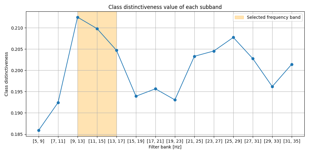
Optimal frequency band for this subject is 9.0 - 15.0 Hz

References

[1]

Class-distinctiveness-based frequency band selection on the Riemannian manifold for oscillatory activity-based BCIs: preliminary results M. S. Yamamoto, F. Lotte, F. Yger, and S. Chevallier. 44th Annual International Conference of the IEEE Engineering in Medicine & Biology Society (EMBC2022), 2022.