Motor imagery classification

Classify motor imagery data with Riemannian geometry [1].

import numpy as np
import pandas as pd
import seaborn as sns
from matplotlib import pyplot as plt

from mne import Epochs, pick_types, events_from_annotations
from mne.io import concatenate_raws
from mne.io.edf import read_raw_edf
from mne.datasets import eegbci
from mne.decoding import CSP
from sklearn.model_selection import cross_val_score, KFold
from sklearn.pipeline import Pipeline
from sklearn.linear_model import LogisticRegression

from pyriemann.classification import MDM, TSclassifier
from pyriemann.estimation import Covariances

Set parameters and read data

# avoid classification of evoked responses by using epochs that start 1s after
# cue onset.
tmin, tmax = 1., 2.
event_id = dict(hands=2, feet=3)
subject = 7
runs = [6, 10, 14]  # motor imagery: hands vs feet

raw_files = [
    read_raw_edf(f, preload=True) for f in eegbci.load_data(subject, runs)
]
raw = concatenate_raws(raw_files)

picks = pick_types(
    raw.info, meg=False, eeg=True, stim=False, eog=False, exclude='bads')
# subsample elecs
picks = picks[::2]

# Apply band-pass filter
raw.filter(7., 35., method='iir', picks=picks)

events, _ = events_from_annotations(raw, event_id=dict(T1=2, T2=3))

# Read epochs (train will be done only between 1 and 2s)
# Testing will be done with a running classifier
epochs = Epochs(
    raw,
    events,
    event_id,
    tmin,
    tmax,
    proj=True,
    picks=picks,
    baseline=None,
    preload=True,
    verbose=False)
labels = epochs.events[:, -1] - 2

# cross validation
cv = KFold(n_splits=10, shuffle=True, random_state=42)
# get epochs
epochs_data_train = 1e6 * epochs.get_data(copy=False)

# compute covariance matrices
cov_data_train = Covariances().transform(epochs_data_train)

Downloading EEGBCI data
Download complete in 08s (7.4 MB)
Extracting EDF parameters from /home/docs/mne_data/MNE-eegbci-data/files/eegmmidb/1.0.0/S007/S007R06.edf...
EDF file detected
Setting channel info structure...
Creating raw.info structure...
Reading 0 ... 19999  =      0.000 ...   124.994 secs...
Extracting EDF parameters from /home/docs/mne_data/MNE-eegbci-data/files/eegmmidb/1.0.0/S007/S007R10.edf...
EDF file detected
Setting channel info structure...
Creating raw.info structure...
Reading 0 ... 19999  =      0.000 ...   124.994 secs...
Extracting EDF parameters from /home/docs/mne_data/MNE-eegbci-data/files/eegmmidb/1.0.0/S007/S007R14.edf...
EDF file detected
Setting channel info structure...
Creating raw.info structure...
Reading 0 ... 19999  =      0.000 ...   124.994 secs...
Filtering a subset of channels. The highpass and lowpass values in the measurement info will not be updated.
Filtering raw data in 3 contiguous segments
Setting up band-pass filter from 7 - 35 Hz

IIR filter parameters
---------------------
Butterworth bandpass zero-phase (two-pass forward and reverse) non-causal filter:
- Filter order 16 (effective, after forward-backward)
- Cutoffs at 7.00, 35.00 Hz: -6.02, -6.02 dB

Used Annotations descriptions: ['T1', 'T2']

Classification with Minimum Distance to Mean

mdm = MDM(metric=dict(mean='riemann', distance='riemann'))

# Use scikit-learn Pipeline with cross_val_score function
scores = cross_val_score(mdm, cov_data_train, labels, cv=cv, n_jobs=1)

# Printing the results
class_balance = np.mean(labels == labels[0])
class_balance = max(class_balance, 1. - class_balance)
print("MDM Classification accuracy: %f / Chance level: %f" % (np.mean(scores),
                                                              class_balance))

MDM Classification accuracy: 0.850000 / Chance level: 0.511111

Classification with Tangent Space Logistic Regression

clf = TSclassifier()
# Use scikit-learn Pipeline with cross_val_score function
scores = cross_val_score(clf, cov_data_train, labels, cv=cv, n_jobs=1)

# Printing the results
class_balance = np.mean(labels == labels[0])
class_balance = max(class_balance, 1. - class_balance)
print("Tangent space Classification accuracy: %f / Chance level: %f" %
      (np.mean(scores), class_balance))

Tangent space Classification accuracy: 0.960000 / Chance level: 0.511111

Classification with CSP + logistic regression

# Assemble a classifier
lr = LogisticRegression()
csp = CSP(n_components=4, reg='ledoit_wolf', log=True)

clf = Pipeline([('CSP', csp), ('LogisticRegression', lr)])
scores = cross_val_score(clf, epochs_data_train, labels, cv=cv, n_jobs=1)

# Printing the results
class_balance = np.mean(labels == labels[0])
class_balance = max(class_balance, 1. - class_balance)
print("CSP + LDA Classification accuracy: %f / Chance level: %f" %
      (np.mean(scores), class_balance))

Computing rank from data with rank=None
    Using tolerance 33 (2.2e-16 eps * 32 dim * 4.7e+15  max singular value)
    Estimated rank (mag): 32
    MAG: rank 32 computed from 32 data channels with 0 projectors
Reducing data rank from 32 -> 32
Estimating covariance using LEDOIT_WOLF
Done.
Computing rank from data with rank=None
    Using tolerance 29 (2.2e-16 eps * 32 dim * 4.1e+15  max singular value)
    Estimated rank (mag): 32
    MAG: rank 32 computed from 32 data channels with 0 projectors
Reducing data rank from 32 -> 32
Estimating covariance using LEDOIT_WOLF
Done.
Computing rank from data with rank=None
    Using tolerance 33 (2.2e-16 eps * 32 dim * 4.6e+15  max singular value)
    Estimated rank (mag): 32
    MAG: rank 32 computed from 32 data channels with 0 projectors
Reducing data rank from 32 -> 32
Estimating covariance using LEDOIT_WOLF
Done.
Computing rank from data with rank=None
    Using tolerance 28 (2.2e-16 eps * 32 dim * 4e+15  max singular value)
    Estimated rank (mag): 32
    MAG: rank 32 computed from 32 data channels with 0 projectors
Reducing data rank from 32 -> 32
Estimating covariance using LEDOIT_WOLF
Done.
Computing rank from data with rank=None
    Using tolerance 34 (2.2e-16 eps * 32 dim * 4.7e+15  max singular value)
    Estimated rank (mag): 32
    MAG: rank 32 computed from 32 data channels with 0 projectors
Reducing data rank from 32 -> 32
Estimating covariance using LEDOIT_WOLF
Done.
Computing rank from data with rank=None
    Using tolerance 27 (2.2e-16 eps * 32 dim * 3.8e+15  max singular value)
    Estimated rank (mag): 32
    MAG: rank 32 computed from 32 data channels with 0 projectors
Reducing data rank from 32 -> 32
Estimating covariance using LEDOIT_WOLF
Done.
Computing rank from data with rank=None
    Using tolerance 33 (2.2e-16 eps * 32 dim * 4.7e+15  max singular value)
    Estimated rank (mag): 32
    MAG: rank 32 computed from 32 data channels with 0 projectors
Reducing data rank from 32 -> 32
Estimating covariance using LEDOIT_WOLF
Done.
Computing rank from data with rank=None
    Using tolerance 29 (2.2e-16 eps * 32 dim * 4e+15  max singular value)
    Estimated rank (mag): 32
    MAG: rank 32 computed from 32 data channels with 0 projectors
Reducing data rank from 32 -> 32
Estimating covariance using LEDOIT_WOLF
Done.
Computing rank from data with rank=None
    Using tolerance 31 (2.2e-16 eps * 32 dim * 4.4e+15  max singular value)
    Estimated rank (mag): 32
    MAG: rank 32 computed from 32 data channels with 0 projectors
Reducing data rank from 32 -> 32
Estimating covariance using LEDOIT_WOLF
Done.
Computing rank from data with rank=None
    Using tolerance 29 (2.2e-16 eps * 32 dim * 4.1e+15  max singular value)
    Estimated rank (mag): 32
    MAG: rank 32 computed from 32 data channels with 0 projectors
Reducing data rank from 32 -> 32
Estimating covariance using LEDOIT_WOLF
Done.
Computing rank from data with rank=None
    Using tolerance 30 (2.2e-16 eps * 32 dim * 4.2e+15  max singular value)
    Estimated rank (mag): 32
    MAG: rank 32 computed from 32 data channels with 0 projectors
Reducing data rank from 32 -> 32
Estimating covariance using LEDOIT_WOLF
Done.
Computing rank from data with rank=None
    Using tolerance 29 (2.2e-16 eps * 32 dim * 4.1e+15  max singular value)
    Estimated rank (mag): 32
    MAG: rank 32 computed from 32 data channels with 0 projectors
Reducing data rank from 32 -> 32
Estimating covariance using LEDOIT_WOLF
Done.
Computing rank from data with rank=None
    Using tolerance 31 (2.2e-16 eps * 32 dim * 4.4e+15  max singular value)
    Estimated rank (mag): 32
    MAG: rank 32 computed from 32 data channels with 0 projectors
Reducing data rank from 32 -> 32
Estimating covariance using LEDOIT_WOLF
Done.
Computing rank from data with rank=None
    Using tolerance 28 (2.2e-16 eps * 32 dim * 4e+15  max singular value)
    Estimated rank (mag): 32
    MAG: rank 32 computed from 32 data channels with 0 projectors
Reducing data rank from 32 -> 32
Estimating covariance using LEDOIT_WOLF
Done.
Computing rank from data with rank=None
    Using tolerance 34 (2.2e-16 eps * 32 dim * 4.7e+15  max singular value)
    Estimated rank (mag): 32
    MAG: rank 32 computed from 32 data channels with 0 projectors
Reducing data rank from 32 -> 32
Estimating covariance using LEDOIT_WOLF
Done.
Computing rank from data with rank=None
    Using tolerance 28 (2.2e-16 eps * 32 dim * 3.9e+15  max singular value)
    Estimated rank (mag): 32
    MAG: rank 32 computed from 32 data channels with 0 projectors
Reducing data rank from 32 -> 32
Estimating covariance using LEDOIT_WOLF
Done.
Computing rank from data with rank=None
    Using tolerance 32 (2.2e-16 eps * 32 dim * 4.5e+15  max singular value)
    Estimated rank (mag): 32
    MAG: rank 32 computed from 32 data channels with 0 projectors
Reducing data rank from 32 -> 32
Estimating covariance using LEDOIT_WOLF
Done.
Computing rank from data with rank=None
    Using tolerance 29 (2.2e-16 eps * 32 dim * 4.1e+15  max singular value)
    Estimated rank (mag): 32
    MAG: rank 32 computed from 32 data channels with 0 projectors
Reducing data rank from 32 -> 32
Estimating covariance using LEDOIT_WOLF
Done.
Computing rank from data with rank=None
    Using tolerance 32 (2.2e-16 eps * 32 dim * 4.5e+15  max singular value)
    Estimated rank (mag): 32
    MAG: rank 32 computed from 32 data channels with 0 projectors
Reducing data rank from 32 -> 32
Estimating covariance using LEDOIT_WOLF
Done.
Computing rank from data with rank=None
    Using tolerance 26 (2.2e-16 eps * 32 dim * 3.7e+15  max singular value)
    Estimated rank (mag): 32
    MAG: rank 32 computed from 32 data channels with 0 projectors
Reducing data rank from 32 -> 32
Estimating covariance using LEDOIT_WOLF
Done.
CSP + LDA Classification accuracy: 0.900000 / Chance level: 0.511111

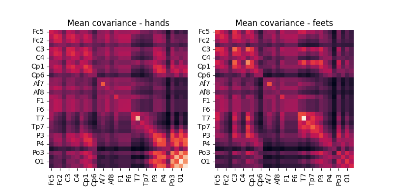
Display MDM centroids

mdm = MDM()
mdm.fit(cov_data_train, labels)

fig, axes = plt.subplots(1, 2, figsize=[8, 4])
ch_names = [ch.replace('.', '') for ch in epochs.ch_names]

df = pd.DataFrame(data=mdm.covmeans_[0], index=ch_names, columns=ch_names)
g = sns.heatmap(
    df, ax=axes[0], square=True, cbar=False, xticklabels=2, yticklabels=2)
g.set_title('Mean covariance - hands')

df = pd.DataFrame(data=mdm.covmeans_[1], index=ch_names, columns=ch_names)
g = sns.heatmap(
    df, ax=axes[1], square=True, cbar=False, xticklabels=2, yticklabels=2)
plt.xticks(rotation='vertical')
plt.yticks(rotation='horizontal')
g.set_title('Mean covariance - feets')

# dirty fix
plt.sca(axes[0])
plt.xticks(rotation='vertical')
plt.yticks(rotation='horizontal')
plt.show()

References

[1]

Multiclass Brain-Computer Interface Classification by Riemannian Geometry A. Barachant, S. Bonnet, M. Congedo, and C. Jutten. IEEE Transactions on Biomedical Engineering, vol. 59, no. 4, p. 920-928, 2012.