Robust covariance estimation

Comparison of robustness of different covariance estimators on a corrupted low-dimensional dataset. See also 1.

# Author: Quentin Barthélemy
#
# License: BSD (3-clause)

import numpy as np
from matplotlib import pyplot as plt
from matplotlib.patches import Ellipse
import matplotlib.transforms as transforms

from pyriemann.estimation import Covariances

def plot_cov_ellipse(ax, cov, n_std=2.5, **kwargs):
    """Inspired by
    https://matplotlib.org/stable/gallery/statistics/confidence_ellipse.html
    """
    pearson = cov[0, 1] / np.sqrt(cov[0, 0] * cov[1, 1])
    ell_radius_x = np.sqrt(1 + pearson)
    ell_radius_y = np.sqrt(1 - pearson)
    ellipse = Ellipse((0, 0), width=ell_radius_x * 2, height=ell_radius_y * 2,
                      facecolor='none', **kwargs)
    scale_x = np.sqrt(cov[0, 0]) * n_std
    scale_y = np.sqrt(cov[1, 1]) * n_std
    transf = transforms.Affine2D().rotate_deg(45).scale(scale_x, scale_y)
    ellipse.set_transform(transf + ax.transData)
    return ax.add_patch(ellipse)


def plot_cov_estimators(ax, X, estimators):
    plot_cov_ellipse(ax, C_ref, edgecolor="C0", label='Reference')
    for i, est in enumerate(estimators):
        C = Covariances(estimator=est).transform(X[np.newaxis, ...])[0]
        plot_cov_ellipse(ax, C, edgecolor=f"C{i+2}", label=est)
    ax.legend(loc='upper left')
    return ax

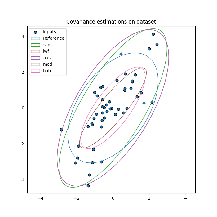
Generate a Gaussian dataset

Input samples are generated from a centered 2D Gaussian distribution considered as the reference.

rs = np.random.RandomState(2023)

n_channels, n_inliers = 2, 50
C_ref = np.array([[1, 0.6], [0.6, 1.5]])
X = C_ref @ rs.randn(n_channels, n_inliers)

Estimate covariance matrices on dataset

Compare reference covariance matrix to different estimators:

• sample covariance matrix (scm),

• Ledoit-Wolf shrunk covariance matrix (lwf),

• oracle approximating shrunk covariance matrix (oas),

• minimum covariance determinant matrix (mcd),

• robust Huber’s M-estimator based covariance matrix (hub).

estimators = ["scm", "lwf", "oas", "mcd", "hub"]

fig, ax = plt.subplots(figsize=(7, 7))
ax.set_title("Covariance estimations on dataset")
ax.scatter(X[0], X[1], c='C0', edgecolors="k", label='Inputs')
ax = plot_cov_estimators(ax, X, estimators)
xlim, ylim = ax.get_xlim(), ax.get_ylim()
min_, max_ = min(xlim[0], ylim[0]), max(xlim[1], ylim[1])
ax.set_xlim(min_, max_)
ax.set_ylim(min_, max_)
plt.show()

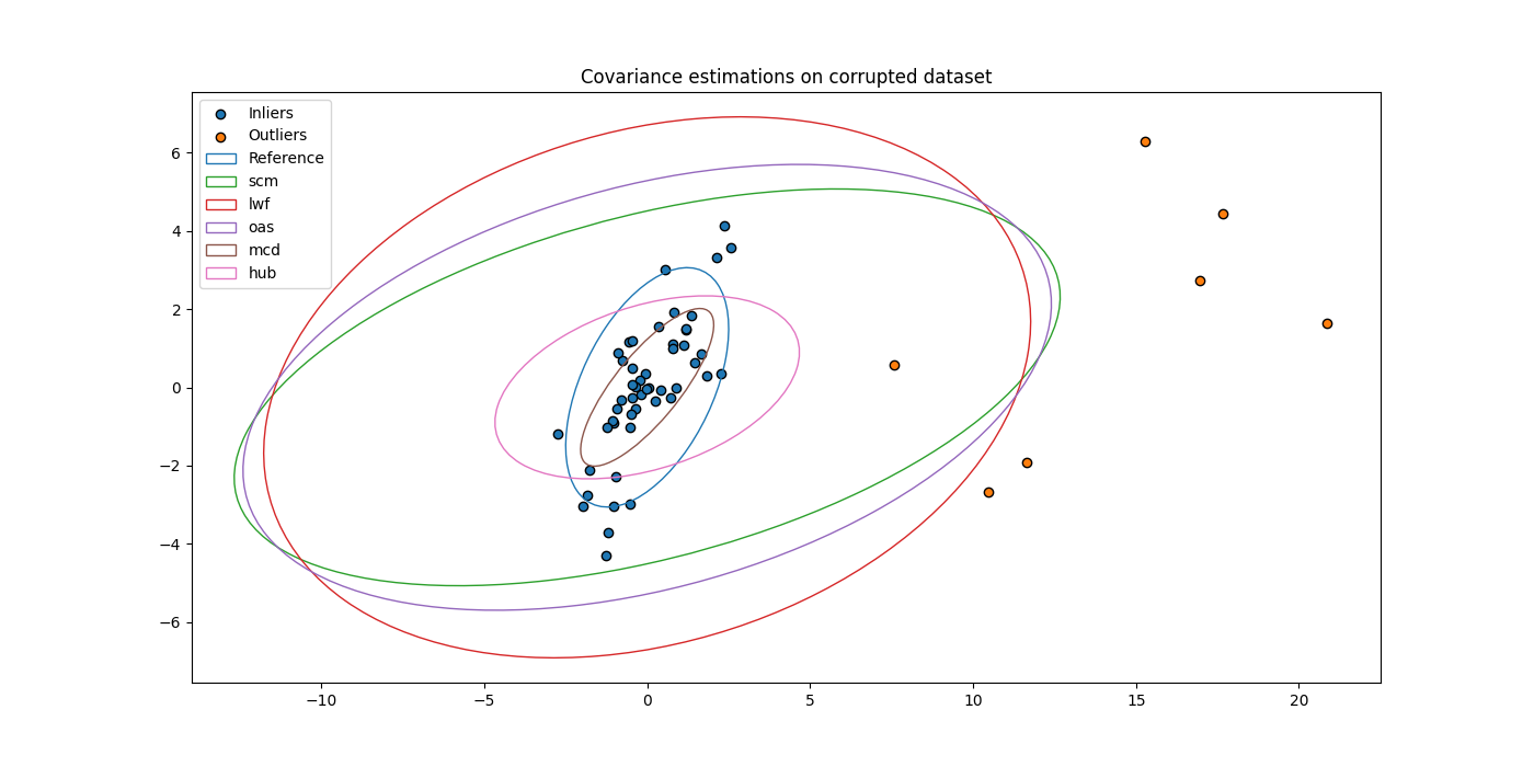
Add outliers to dataset

Outliers are added to the dataset.

n_outliers = 7
mu, scale = np.array([15, 1]), 5
Xout = mu[:, np.newaxis] + scale * rs.randn(n_channels, n_outliers)
X = np.concatenate((X, Xout), axis=1)

Estimate covariance matrices on corrupted dataset

Compare robustness of the different estimators.

fig, ax = plt.subplots(figsize=(14, 7))
ax.set_title("Covariance estimations on corrupted dataset")
ax.scatter(X[0, :n_inliers], X[1, :n_inliers], c='C0', edgecolors="k",
           label='Inliers')
ax.scatter(X[0, n_inliers:], X[1, n_inliers:], c='C1', edgecolors="k",
           label='Outliers')
ax = plot_cov_estimators(ax, X, estimators)
plt.show()

References

1

https://scikit-learn.org/stable/auto_examples/covariance/plot_mahalanobis_distances.html # noqa