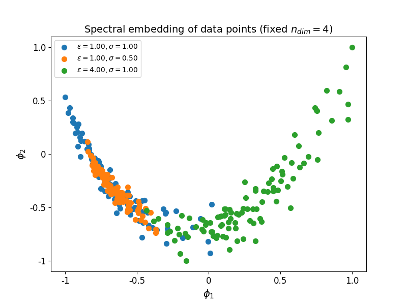
Sample from the Riemannian Gaussian distribution in the SPD manifold

Spectral embedding of samples from the Riemannian Gaussian distribution with different centerings and dispersions.

# Authors: Pedro Rodrigues <pedro.rodrigues@melix.org>
#
# License: BSD (3-clause)

import numpy as np
import matplotlib.pyplot as plt

from pyriemann.embedding import SpectralEmbedding
from pyriemann.datasets import sample_gaussian_spd, generate_random_spd_matrix


print(__doc__)

Set parameters for sampling from the Riemannian Gaussian distribution

n_matrices = 100  # how many SPD matrices to generate
n_dim = 2  # number of dimensions of the SPD matrices
sigma = 1.0  # dispersion of the Gaussian distribution
epsilon = 4.0  # parameter for controlling the distance between centers
random_state = 42  # ensure reproducibility

# Generate the samples on three different conditions
mean = generate_random_spd_matrix(n_dim)  # random reference point

samples_1 = sample_gaussian_spd(n_matrices=n_matrices,
                                mean=mean,
                                sigma=sigma,
                                random_state=random_state)
samples_2 = sample_gaussian_spd(n_matrices=n_matrices,
                                mean=mean,
                                sigma=sigma/2,
                                random_state=random_state)
samples_3 = sample_gaussian_spd(n_matrices=n_matrices,
                                mean=epsilon*mean,
                                sigma=sigma,
                                random_state=random_state)

# Stack all of the samples into one data array for the embedding
samples = np.concatenate([samples_1, samples_2, samples_3])
labels = np.array(n_matrices*[1] + n_matrices*[2] + n_matrices*[3])

Apply the spectral embedding over the SPD matrices

lapl = SpectralEmbedding(metric='riemann', n_components=2)
embd = lapl.fit_transform(X=samples)

Plot the results

fig, ax = plt.subplots(figsize=(8, 6))

colors = {1: 'C0', 2: 'C1', 3: 'C2'}
for i in range(len(samples)):
    ax.scatter(embd[i, 0], embd[i, 1], c=colors[labels[i]], s=50)
ax.scatter([], [], c='C0', s=50, label=r'$\varepsilon = 1.00, \sigma = 1.00$')
ax.scatter([], [], c='C1', s=50, label=r'$\varepsilon = 1.00, \sigma = 0.50$')
ax.scatter([], [], c='C2', s=50, label=r'$\varepsilon = 4.00, \sigma = 1.00$')
ax.set_xticks([-1, -0.5, 0, 0.5, 1.0])
ax.set_xticklabels([-1, -0.5, 0, 0.5, 1.0], fontsize=12)
ax.set_yticks([-1, -0.5, 0, 0.5, 1.0])
ax.set_yticklabels([-1, -0.5, 0, 0.5, 1.0], fontsize=12)
ax.set_title(r'Spectral embedding of data points (fixed $n_{dim} = 4$)',
             fontsize=14)
ax.set_xlabel(r'$\phi_1$', fontsize=14)
ax.set_ylabel(r'$\phi_2$', fontsize=14)
ax.legend()

plt.show()