Note
Click here to download the full example code
Visualization of SSVEP-based BCI Classification in Tangent Space
Project extended covariance matrices of SSVEP-based BCI in the tangent space, using principal geodesic analysis (PGA).
You should have a look to “Offline SSVEP-based BCI Multiclass Prediction” before this example.
# Authors: Quentin Barthélemy, Emmanuel Kalunga and Sylvain Chevallier
#
# License: BSD (3-clause)
import numpy as np
import matplotlib.pyplot as plt
from matplotlib.animation import FuncAnimation
from mne import find_events, Epochs, make_fixed_length_epochs
from mne.io import Raw
from sklearn.pipeline import make_pipeline
from sklearn.decomposition import PCA
from pyriemann.estimation import BlockCovariances
from pyriemann.classification import MDM
from pyriemann.tangentspace import TangentSpace
from pyriemann.utils.viz import _add_alpha
from helpers.ssvep_helpers import download_data, extend_signal
clabel = ['resting-state', '13 Hz', '17 Hz', '21 Hz']
clist = plt.cm.viridis(np.array([0, 1, 2, 3])/3)
cmap = "viridis"
def plot_pga(ax, data, labels, centers):
sc = ax.scatter(data[:, 0], data[:, 1], c=labels, marker='P', cmap=cmap)
ax.scatter(
centers[:, 0], centers[:, 1], c=clist, marker='o', s=100, cmap=cmap
)
ax.set(xlabel='PGA, 1st axis', ylabel='PGA, 2nd axis')
for i in range(len(clabel)):
ax.scatter([], [], color=clist[i], marker='o', s=50, label=clabel[i])
ax.legend(loc='upper right')
return sc
Load EEG and extract covariance matrices for SSVEP
frequencies = [13, 17, 21]
freq_band = 0.1
events_id = {'13 Hz': 2, '17 Hz': 4, '21 Hz': 3, 'resting-state': 1}
duration = 2.5 # duration of epochs
interval = 0.25 # interval between successive epochs for online processing
# Subject 12: first 4 sessions for training, last session for test
# Training set
raw = Raw(download_data(subject=12, session=1), preload=True, verbose=False)
events = find_events(raw, shortest_event=0, verbose=False)
raw = raw.pick_types(eeg=True)
ch_count = len(raw.info['ch_names'])
raw_ext = extend_signal(raw, frequencies, freq_band)
epochs = Epochs(
raw_ext, events, events_id, tmin=2, tmax=5, baseline=None, verbose=False)
x_train = BlockCovariances(
estimator='lwf', block_size=ch_count).transform(epochs.get_data())
y_train = events[:, 2]
# Testing set
raw = Raw(download_data(subject=12, session=4), preload=True, verbose=False)
raw = raw.pick_types(eeg=True)
raw_ext = extend_signal(raw, frequencies, freq_band)
epochs = make_fixed_length_epochs(
raw_ext, duration=duration, overlap=duration - interval, verbose=False)
x_test = BlockCovariances(
estimator='lwf', block_size=ch_count).transform(epochs.get_data())
Creating RawArray with float64 data, n_channels=24, n_times=92384
Range : 0 ... 92383 = 0.000 ... 360.871 secs
Ready.
Using data from preloaded Raw for 32 events and 769 original time points ...
0 bad epochs dropped
0%| | 0.00/5.35M [00:00<?, ?B/s]
1%|▏ | 31.7k/5.35M [00:00<01:08, 77.3kB/s]
1%|▍ | 64.5k/5.35M [00:00<00:41, 126kB/s]
2%|▉ | 130k/5.35M [00:00<00:22, 230kB/s]
3%|█▎ | 179k/5.35M [00:00<00:19, 262kB/s]
5%|█▊ | 245k/5.35M [00:01<00:16, 319kB/s]
5%|██ | 281k/5.35M [00:01<00:17, 295kB/s]
6%|██▌ | 343k/5.35M [00:01<00:15, 334kB/s]
8%|██▉ | 409k/5.35M [00:01<00:13, 367kB/s]
9%|███▍ | 474k/5.35M [00:01<00:12, 390kB/s]
10%|███▉ | 540k/5.35M [00:01<00:11, 405kB/s]
11%|████▎ | 589k/5.35M [00:01<00:12, 383kB/s]
12%|████▊ | 654k/5.35M [00:02<00:11, 399kB/s]
13%|█████▏ | 720k/5.35M [00:02<00:11, 411kB/s]
15%|█████▋ | 785k/5.35M [00:02<00:10, 419kB/s]
16%|██████▏ | 851k/5.35M [00:02<00:10, 426kB/s]
17%|██████▋ | 916k/5.35M [00:02<00:10, 430kB/s]
18%|███████▏ | 982k/5.35M [00:02<00:10, 434kB/s]
20%|███████▍ | 1.05M/5.35M [00:02<00:09, 435kB/s]
21%|███████▉ | 1.11M/5.35M [00:03<00:09, 438kB/s]
22%|████████▎ | 1.16M/5.35M [00:03<00:10, 405kB/s]
23%|████████▋ | 1.23M/5.35M [00:03<00:09, 416kB/s]
24%|█████████▏ | 1.29M/5.35M [00:03<00:09, 423kB/s]
26%|█████████▊ | 1.38M/5.35M [00:03<00:08, 461kB/s]
27%|██████████▏ | 1.44M/5.35M [00:03<00:08, 455kB/s]
28%|██████████▋ | 1.51M/5.35M [00:03<00:08, 450kB/s]
29%|███████████▏ | 1.57M/5.35M [00:04<00:08, 448kB/s]
30%|███████████▌ | 1.62M/5.35M [00:04<00:09, 413kB/s]
32%|███████████▉ | 1.69M/5.35M [00:04<00:08, 422kB/s]
32%|████████████▎ | 1.73M/5.35M [00:04<00:09, 382kB/s]
34%|████████████▊ | 1.80M/5.35M [00:04<00:08, 412kB/s]
35%|█████████████▎ | 1.87M/5.35M [00:04<00:08, 420kB/s]
36%|█████████████▋ | 1.93M/5.35M [00:05<00:08, 427kB/s]
37%|██████████████▏ | 2.00M/5.35M [00:05<00:07, 431kB/s]
39%|██████████████▋ | 2.06M/5.35M [00:05<00:07, 435kB/s]
40%|███████████████ | 2.13M/5.35M [00:05<00:07, 436kB/s]
41%|███████████████▋ | 2.21M/5.35M [00:05<00:06, 470kB/s]
43%|████████████████▏ | 2.28M/5.35M [00:05<00:06, 462kB/s]
44%|████████████████▋ | 2.34M/5.35M [00:05<00:06, 456kB/s]
45%|█████████████████ | 2.41M/5.35M [00:06<00:06, 452kB/s]
46%|█████████████████▌ | 2.47M/5.35M [00:06<00:06, 449kB/s]
47%|██████████████████ | 2.54M/5.35M [00:06<00:06, 446kB/s]
49%|██████████████████▍ | 2.60M/5.35M [00:06<00:06, 444kB/s]
50%|██████████████████▉ | 2.67M/5.35M [00:06<00:06, 443kB/s]
51%|███████████████████▍ | 2.74M/5.35M [00:06<00:05, 443kB/s]
52%|███████████████████▉ | 2.80M/5.35M [00:06<00:05, 442kB/s]
54%|████████████████████▎ | 2.87M/5.35M [00:07<00:05, 442kB/s]
55%|████████████████████▊ | 2.93M/5.35M [00:07<00:05, 441kB/s]
56%|█████████████████████▎ | 3.00M/5.35M [00:07<00:05, 440kB/s]
57%|█████████████████████▊ | 3.06M/5.35M [00:07<00:05, 439kB/s]
58%|██████████████████████▏ | 3.13M/5.35M [00:07<00:05, 439kB/s]
60%|██████████████████████▋ | 3.19M/5.35M [00:07<00:04, 439kB/s]
61%|███████████████████████▏ | 3.26M/5.35M [00:07<00:04, 439kB/s]
62%|███████████████████████▌ | 3.32M/5.35M [00:08<00:04, 439kB/s]
63%|████████████████████████ | 3.39M/5.35M [00:08<00:04, 439kB/s]
65%|████████████████████████▌ | 3.46M/5.35M [00:08<00:04, 439kB/s]
66%|█████████████████████████ | 3.52M/5.35M [00:08<00:04, 439kB/s]
67%|█████████████████████████▍ | 3.59M/5.35M [00:08<00:04, 439kB/s]
68%|█████████████████████████▉ | 3.65M/5.35M [00:08<00:03, 439kB/s]
69%|██████████████████████████▍ | 3.72M/5.35M [00:09<00:03, 439kB/s]
71%|██████████████████████████▊ | 3.78M/5.35M [00:09<00:03, 440kB/s]
72%|███████████████████████████▎ | 3.85M/5.35M [00:09<00:03, 440kB/s]
73%|███████████████████████████▉ | 3.93M/5.35M [00:09<00:03, 473kB/s]
75%|████████████████████████████▍ | 4.00M/5.35M [00:09<00:02, 462kB/s]
76%|████████████████████████████▊ | 4.06M/5.35M [00:09<00:02, 455kB/s]
77%|█████████████████████████████▎ | 4.13M/5.35M [00:09<00:02, 450kB/s]
78%|█████████████████████████████▊ | 4.19M/5.35M [00:10<00:02, 445kB/s]
79%|██████████████████████████████▏ | 4.24M/5.35M [00:10<00:02, 411kB/s]
81%|██████████████████████████████▌ | 4.31M/5.35M [00:10<00:02, 419kB/s]
82%|███████████████████████████████ | 4.37M/5.35M [00:10<00:02, 425kB/s]
83%|███████████████████████████████▌ | 4.44M/5.35M [00:10<00:02, 429kB/s]
84%|███████████████████████████████▉ | 4.50M/5.35M [00:10<00:01, 433kB/s]
85%|████████████████████████████████▍ | 4.57M/5.35M [00:10<00:01, 435kB/s]
87%|████████████████████████████████▉ | 4.64M/5.35M [00:11<00:01, 437kB/s]
88%|█████████████████████████████████▍ | 4.70M/5.35M [00:11<00:01, 438kB/s]
89%|█████████████████████████████████▊ | 4.77M/5.35M [00:11<00:01, 438kB/s]
90%|██████████████████████████████████▎ | 4.83M/5.35M [00:11<00:01, 439kB/s]
92%|██████████████████████████████████▊ | 4.90M/5.35M [00:11<00:01, 439kB/s]
93%|███████████████████████████████████▎ | 4.96M/5.35M [00:11<00:00, 439kB/s]
94%|███████████████████████████████████▋ | 5.03M/5.35M [00:12<00:00, 438kB/s]
95%|████████████████████████████████████▏ | 5.09M/5.35M [00:12<00:00, 439kB/s]
96%|████████████████████████████████████▋ | 5.16M/5.35M [00:12<00:00, 439kB/s]
98%|█████████████████████████████████████ | 5.23M/5.35M [00:12<00:00, 439kB/s]
99%|█████████████████████████████████████▌| 5.29M/5.35M [00:12<00:00, 439kB/s]
0%| | 0.00/5.35M [00:00<?, ?B/s]
100%|█████████████████████████████████████| 5.35M/5.35M [00:00<00:00, 13.7GB/s]
Creating RawArray with float64 data, n_channels=24, n_times=148544
Range : 0 ... 148543 = 0.000 ... 580.246 secs
Ready.
Using data from preloaded Raw for 2312 events and 640 original time points ...
0 bad epochs dropped
Classification with minimum distance to mean (MDM)
Classification for a 4-class SSVEP BCI, including resting-state class.
print("Number of training trials: {}".format(len(x_train)))
mdm = MDM(metric=dict(mean='riemann', distance='riemann'))
mdm.fit(x_train, y_train)
Number of training trials: 32
MDM(metric={'distance': 'riemann', 'mean': 'riemann'})
Projection in tangent space with principal geodesic analysis (PGA)
Project covariance matrices from the Riemannian manifold into the Euclidean tangent space at the grand average, and apply a principal component analysis (PCA) to obtain an unsupervised dimension reduction 1.
pga = make_pipeline(
TangentSpace(metric="riemann", tsupdate=False),
PCA(n_components=2)
)
ts_train = pga.fit_transform(x_train)
ts_means = pga.transform(np.array(mdm.covmeans_))
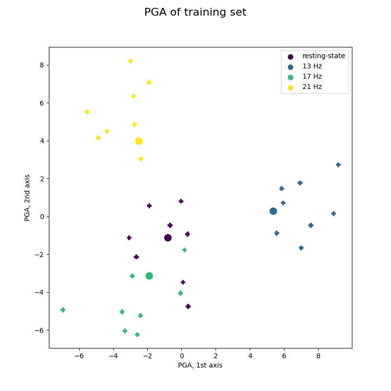
Offline training of MDM visualized by PGA
These figures show the trajectory on the tangent space taken by covariance matrices during a 4-class SSVEP experiment, and how they are classified epoch by epoch.
This figure reproduces Fig 3(c) of reference 2, showing training trials of best subject.
fig, ax = plt.subplots(figsize=(8, 8))
fig.suptitle('PGA of training set', fontsize=16)
plot_pga(ax, ts_train, y_train, ts_means)
plt.show()
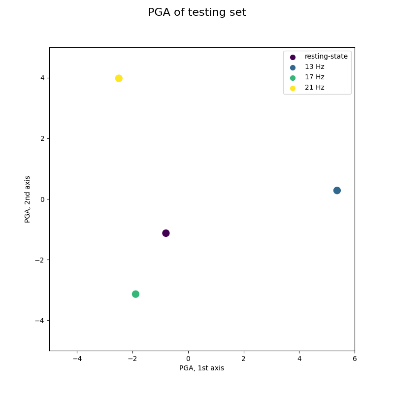
Online classification by MDM visualized by PGA
This figure reproduces Fig 6 of reference 2, with an animation to imitate an online acquisition, processing and classification of EEG time-series.
Warning: 2 uses a curved based online classification, while a single trial classification is used here.
# Prepare data for online classification
test_visu = 50 # nb of matrices to display simultaneously
colors, ts_visu = [], np.empty([0, 2])
alphas = np.linspace(0, 1, test_visu)
fig, ax = plt.subplots(figsize=(8, 8))
fig.suptitle('PGA of testing set', fontsize=16)
pl = plot_pga(ax, ts_visu, colors, ts_means)
pl.axes.set_xlim(-5, 6)
pl.axes.set_ylim(-5, 5)
(-5.0, 5.0)
# Prepare animation for online classification
def online_classify(t):
global colors, ts_visu
# Online classification
y = mdm.predict(x_test[np.newaxis, t])
color = clist[int(y[0] - 1)]
ts_test = pga.transform(x_test[np.newaxis, t])
# Update data
colors.append(color)
ts_visu = np.vstack((ts_visu, ts_test))
if len(ts_visu) > test_visu:
colors.pop(0)
ts_visu = ts_visu[1:]
colors = _add_alpha(colors, alphas)
# Update plot
pl.set_offsets(np.c_[ts_visu[:, 0], ts_visu[:, 1]])
pl.set_color(colors)
return pl
interval_display = 1.0 # can be changed for a slower display
visu = FuncAnimation(fig, online_classify,
frames=range(0, len(x_test)),
interval=interval_display, blit=False, repeat=False)
# Plot online classification
# Plot complete visu: a dynamic display is required
plt.show()
# Plot only 10s, for animated documentation
try:
from IPython.display import HTML
except ImportError:
raise ImportError("Install IPython to plot animation in documentation")
plt.rcParams["animation.embed_limit"] = 10
HTML(visu.to_jshtml(fps=5, default_mode='loop'))
Animation size has reached 10525072 bytes, exceeding the limit of 10485760.0. If you're sure you want a larger animation embedded, set the animation.embed_limit rc parameter to a larger value (in MB). This and further frames will be dropped.