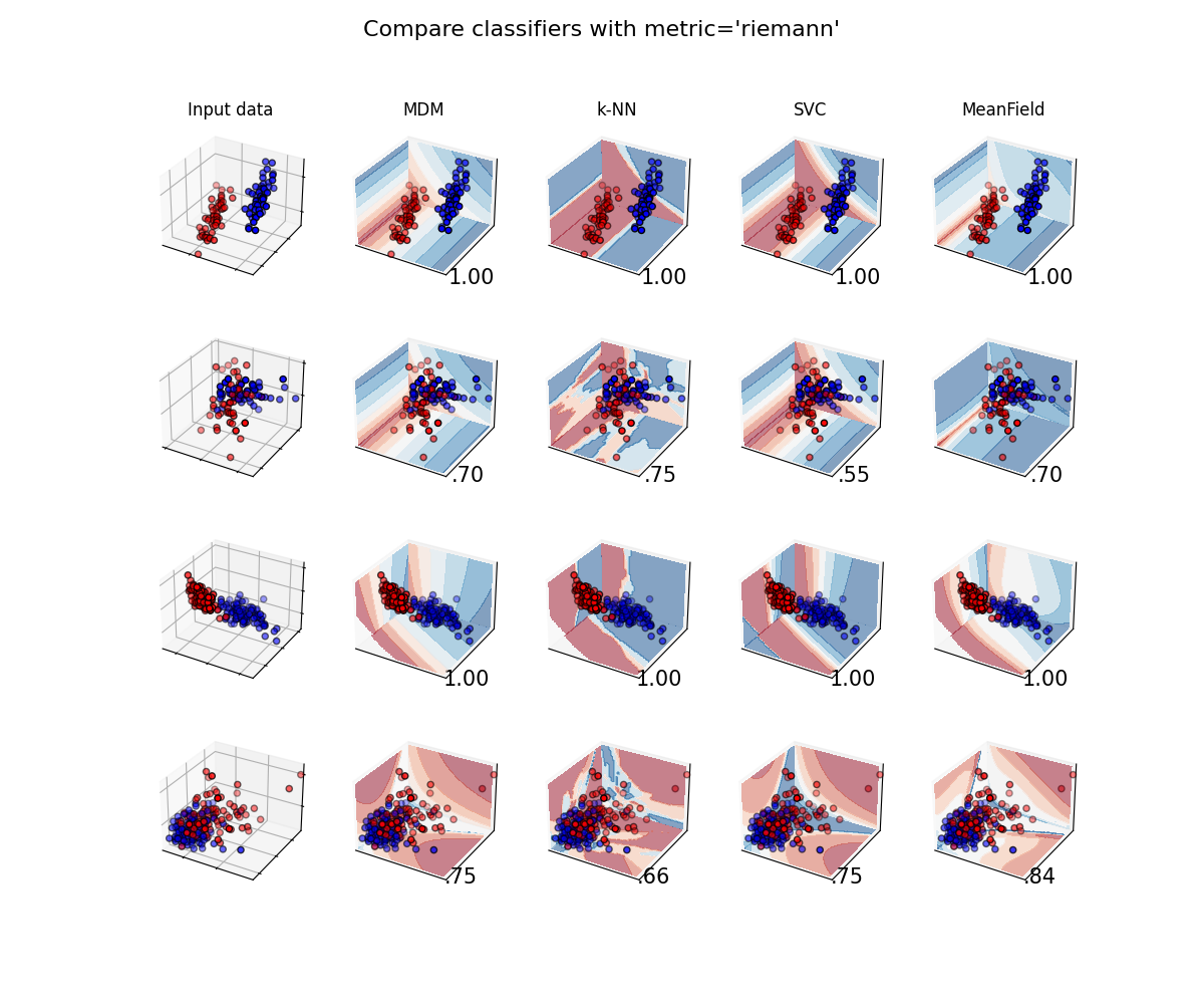
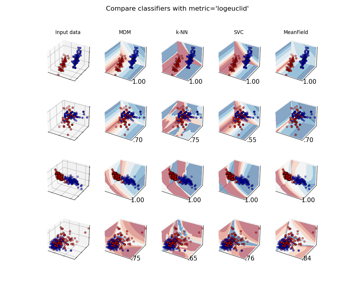
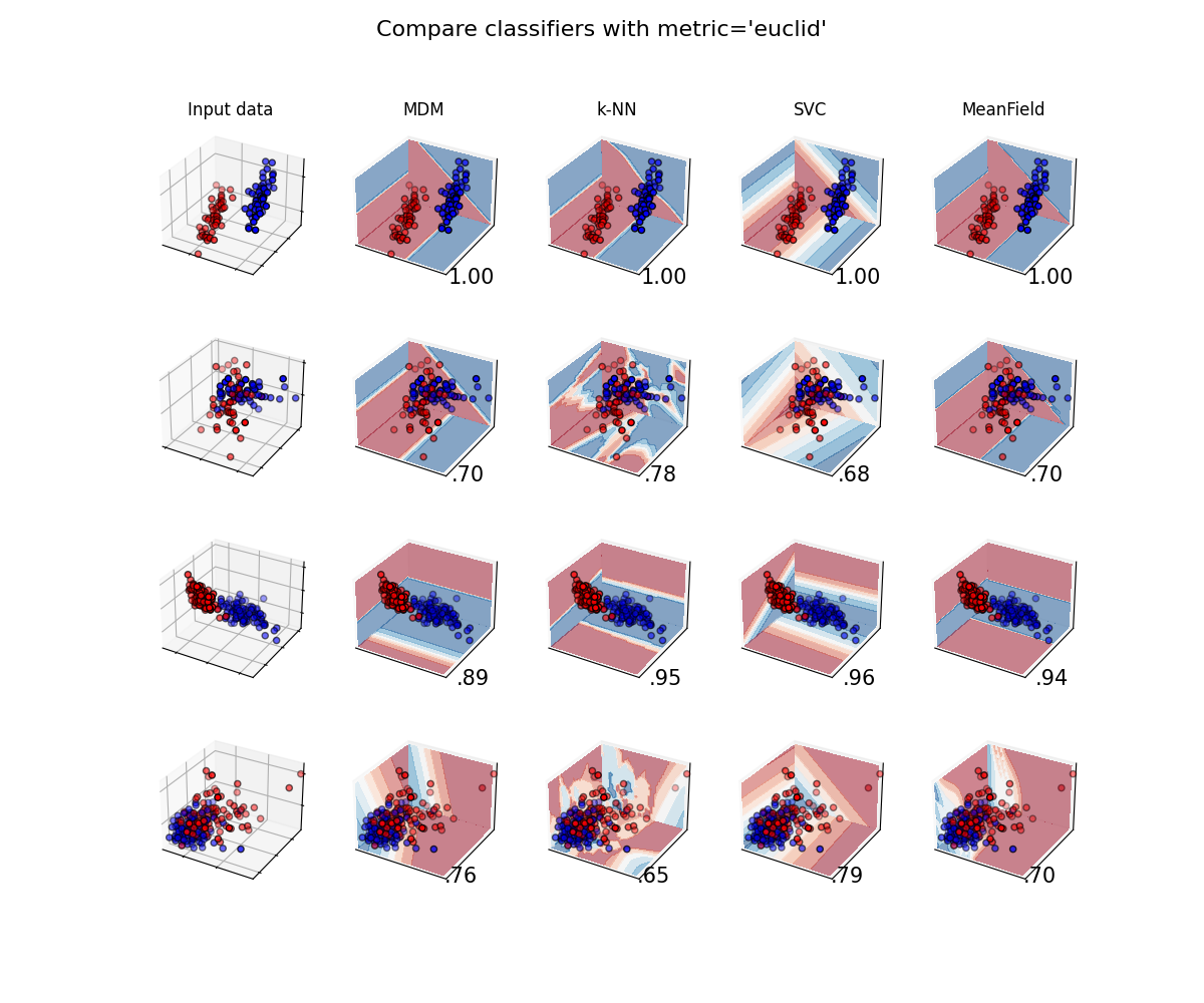
Classifier comparison

A comparison of several classifiers on low-dimensional synthetic datasets, adapted to SPD matrices from 1. The point of this example is to illustrate the nature of decision boundaries of different classifiers, used with different metrics 2. This should be taken with a grain of salt, as the intuition conveyed by these examples does not necessarily carry over to real datasets.

The 3D plots show training matrices in solid colors and testing matrices semi-transparent. The lower right shows the classification accuracy on the test set.

# Authors: Quentin Barthélemy
#
# License: BSD (3-clause)

from functools import partial
from time import time

import numpy as np
import matplotlib.pyplot as plt
from matplotlib.colors import ListedColormap
from sklearn.model_selection import train_test_split

from pyriemann.datasets import make_covariances, make_gaussian_blobs
from pyriemann.classification import (
    MDM,
    KNearestNeighbor,
    SVC,
    MeanField,
)

@partial(np.vectorize, excluded=['clf'])
def get_proba(cov_00, cov_01, cov_11, clf):
    cov = np.array([[cov_00, cov_01], [cov_01, cov_11]])
    with np.testing.suppress_warnings() as sup:
        sup.filter(RuntimeWarning)
        return clf.predict_proba(cov[np.newaxis, ...])[0, 1]


def plot_classifiers(metric):
    figure = plt.figure(figsize=(12, 10))
    figure.suptitle(f"Compare classifiers with metric='{metric}'", fontsize=16)
    i = 1

    # iterate over datasets
    for ds_cnt, (X, y) in enumerate(datasets):
        # split dataset into training and test part
        X_train, X_test, y_train, y_test = train_test_split(
            X, y, test_size=0.4, random_state=42
        )

        x_min, x_max = X[:, 0, 0].min(), X[:, 0, 0].max()
        y_min, y_max = X[:, 0, 1].min(), X[:, 0, 1].max()
        z_min, z_max = X[:, 1, 1].min(), X[:, 1, 1].max()

        # just plot the dataset first
        ax = plt.subplot(n_datasets, n_classifs + 1, i, projection='3d')
        if ds_cnt == 0:
            ax.set_title("Input data")
        # Plot the training points
        ax.scatter(
            X_train[:, 0, 0],
            X_train[:, 0, 1],
            X_train[:, 1, 1],
            c=y_train,
            cmap=cm_bright,
            edgecolors="k"
        )
        # Plot the testing points
        ax.scatter(
            X_test[:, 0, 0],
            X_test[:, 0, 1],
            X_test[:, 1, 1],
            c=y_test,
            cmap=cm_bright,
            alpha=0.6,
            edgecolors="k"
        )
        ax.set_xlim(x_min, x_max)
        ax.set_ylim(y_min, y_max)
        ax.set_zlim(z_min, z_max)
        ax.set_xticklabels(())
        ax.set_yticklabels(())
        ax.set_zticklabels(())
        i += 1

        rx = np.arange(x_min, x_max, (x_max - x_min) / 50)
        ry = np.arange(y_min, y_max, (y_max - y_min) / 50)
        rz = np.arange(z_min, z_max, (z_max - z_min) / 50)

        print(f"Dataset n°{ds_cnt+1}")

        # iterate over classifiers
        for name, clf in zip(names, classifiers):
            ax = plt.subplot(n_datasets, n_classifs + 1, i, projection='3d')

            clf.set_params(**{'metric': metric})
            t0 = time()
            clf.fit(X_train, y_train)
            t1 = time() - t0

            t0 = time()
            score = clf.score(X_test, y_test)
            t2 = time() - t0

            print(
                f" {name}:\n  training time={t1:.5f}\n  test time    ={t2:.5f}"
            )

            # Plot the decision boundaries for horizontal 2D planes going
            # through the mean value of the third coordinates
            xx, yy = np.meshgrid(rx, ry)
            zz = get_proba(xx, yy, X[:, 1, 1].mean()*np.ones_like(xx), clf=clf)
            zz = np.ma.masked_where(~np.isfinite(zz), zz)
            ax.contourf(xx, yy, zz, zdir='z', offset=z_min, cmap=cm, alpha=0.5)

            xx, zz = np.meshgrid(rx, rz)
            yy = get_proba(xx, X[:, 0, 1].mean()*np.ones_like(xx), zz, clf=clf)
            yy = np.ma.masked_where(~np.isfinite(yy), yy)
            ax.contourf(xx, yy, zz, zdir='y', offset=y_max, cmap=cm, alpha=0.5)

            yy, zz = np.meshgrid(ry, rz)
            xx = get_proba(X[:, 0, 0].mean()*np.ones_like(yy), yy, zz, clf=clf)
            xx = np.ma.masked_where(~np.isfinite(xx), xx)
            ax.contourf(xx, yy, zz, zdir='x', offset=x_min, cmap=cm, alpha=0.5)

            # Plot the training points
            ax.scatter(
                X_train[:, 0, 0],
                X_train[:, 0, 1],
                X_train[:, 1, 1],
                c=y_train,
                cmap=cm_bright,
                edgecolors="k"
            )
            # Plot the testing points
            ax.scatter(
                X_test[:, 0, 0],
                X_test[:, 0, 1],
                X_test[:, 1, 1],
                c=y_test,
                cmap=cm_bright,
                edgecolors="k",
                alpha=0.6
            )

            if ds_cnt == 0:
                ax.set_title(name)
            ax.text(
                1.3 * x_max,
                y_min,
                z_min,
                ("%.2f" % score).lstrip("0"),
                size=15,
                horizontalalignment="right",
                verticalalignment="bottom"
            )
            ax.set_xlim(x_min, x_max)
            ax.set_ylim(y_min, y_max)
            ax.set_zlim(z_min, z_max)
            ax.set_xticks(())
            ax.set_yticks(())
            ax.set_zticks(())

            i += 1

    plt.show()

Classifiers and Datasets

names = [
    "MDM",
    "k-NN",
    "SVC",
    "MeanField",
]
classifiers = [
    MDM(),
    KNearestNeighbor(n_neighbors=3),
    SVC(probability=True),
    MeanField(power_list=[-1, 0, 1]),
]
n_classifs = len(classifiers)

rs = np.random.RandomState(2022)
n_matrices, n_channels = 50, 2
y = np.concatenate([np.zeros(n_matrices), np.ones(n_matrices)])

datasets = [
    (
        np.concatenate([
            make_covariances(
                n_matrices, n_channels, rs, evals_mean=10, evals_std=1
            ),
            make_covariances(
                n_matrices, n_channels, rs, evals_mean=15, evals_std=1
            )
        ]),
        y
    ),
    (
        np.concatenate([
            make_covariances(
                n_matrices, n_channels, rs, evals_mean=10, evals_std=2
            ),
            make_covariances(
                n_matrices, n_channels, rs, evals_mean=12, evals_std=2
            )
        ]),
        y
    ),
    make_gaussian_blobs(
        2*n_matrices, n_channels, random_state=rs, class_sep=1., class_disp=.2,
        n_jobs=4
    ),
    make_gaussian_blobs(
        2*n_matrices, n_channels, random_state=rs, class_sep=.5, class_disp=.5,
        n_jobs=4
    )
]
n_datasets = len(datasets)

cm = plt.cm.RdBu
cm_bright = ListedColormap(["#FF0000", "#0000FF"])

Classifiers with Riemannian metric

plot_classifiers("riemann")

Dataset n°1
 MDM:
  training time=0.00224
  test time    =0.00698
 k-NN:
  training time=0.00007
  test time    =0.15169
 SVC:
  training time=0.00378
  test time    =0.00158
 MeanField:
  training time=0.01857
  test time    =0.02697
Dataset n°2
 MDM:
  training time=0.00219
  test time    =0.00697
 k-NN:
  training time=0.00006
  test time    =0.15051
 SVC:
  training time=0.00430
  test time    =0.00155
 MeanField:
  training time=0.01853
  test time    =0.02723
Dataset n°3
 MDM:
  training time=0.00534
  test time    =0.01304
 k-NN:
  training time=0.00005
  test time    =0.44538
 SVC:
  training time=0.00709
  test time    =0.00180
 MeanField:
  training time=0.02700
  test time    =0.05292
Dataset n°4
 MDM:
  training time=0.00662
  test time    =0.01321
 k-NN:
  training time=0.00005
  test time    =0.44173
 SVC:
  training time=0.00820
  test time    =0.00195
/home/docs/checkouts/readthedocs.org/user_builds/pyriemann/envs/v0.4/lib/python3.7/site-packages/numpy/lib/function_base.py:2246: RuntimeWarning: invalid value encountered in func (vectorized)
  outputs = ufunc(*inputs)
/home/docs/checkouts/readthedocs.org/user_builds/pyriemann/envs/v0.4/lib/python3.7/site-packages/numpy/lib/function_base.py:2246: RuntimeWarning: invalid value encountered in func (vectorized)
  outputs = ufunc(*inputs)
 MeanField:
  training time=0.02767
  test time    =0.05270

Classifiers with Log-Euclidean metric

plot_classifiers("logeuclid")

Dataset n°1
 MDM:
  training time=0.00088
  test time    =0.01053
 k-NN:
  training time=0.00007
  test time    =0.20826
 SVC:
  training time=0.00215
  test time    =0.00135
 MeanField:
  training time=0.01852
  test time    =0.03861
Dataset n°2
 MDM:
  training time=0.00093
  test time    =0.01069
 k-NN:
  training time=0.00006
  test time    =0.20739
 SVC:
  training time=0.00237
  test time    =0.00138
 MeanField:
  training time=0.01840
  test time    =0.03863
Dataset n°3
 MDM:
  training time=0.00116
  test time    =0.02075
 k-NN:
  training time=0.00006
  test time    =0.67098
 SVC:
  training time=0.00279
  test time    =0.00149
 MeanField:
  training time=0.02781
  test time    =0.07671
Dataset n°4
 MDM:
  training time=0.00118
  test time    =0.02058
 k-NN:
  training time=0.00005
  test time    =0.67740
 SVC:
  training time=0.00400
  test time    =0.00160
/home/docs/checkouts/readthedocs.org/user_builds/pyriemann/envs/v0.4/lib/python3.7/site-packages/numpy/lib/function_base.py:2246: RuntimeWarning: invalid value encountered in func (vectorized)
  outputs = ufunc(*inputs)
/home/docs/checkouts/readthedocs.org/user_builds/pyriemann/envs/v0.4/lib/python3.7/site-packages/numpy/lib/function_base.py:2246: RuntimeWarning: invalid value encountered in func (vectorized)
  outputs = ufunc(*inputs)
 MeanField:
  training time=0.02854
  test time    =0.07650

Classifiers with Euclidean metric

plot_classifiers("euclid")

Dataset n°1
 MDM:
  training time=0.00041
  test time    =0.00202
 k-NN:
  training time=0.00007
  test time    =0.04523
 SVC:
  training time=0.00148
  test time    =0.00079
 MeanField:
  training time=0.01832
  test time    =0.01050
Dataset n°2
 MDM:
  training time=0.00037
  test time    =0.00201
 k-NN:
  training time=0.00006
  test time    =0.04581
 SVC:
  training time=0.00258
  test time    =0.00082
 MeanField:
  training time=0.02015
  test time    =0.01046
Dataset n°3
 MDM:
  training time=0.00037
  test time    =0.00331
 k-NN:
  training time=0.00005
  test time    =0.13844
 SVC:
  training time=0.00179
  test time    =0.00085
 MeanField:
  training time=0.02678
  test time    =0.01953
Dataset n°4
 MDM:
  training time=0.00036
  test time    =0.00392
 k-NN:
  training time=0.00005
  test time    =0.13824
 SVC:
  training time=0.00298
  test time    =0.00093
 MeanField:
  training time=0.02838
  test time    =0.01951

References

1

https://scikit-learn.org/stable/auto_examples/classification/plot_classifier_comparison.html # noqa

2

Review of Riemannian distances and divergences, applied to SSVEP-based BCI S. Chevallier, E. K. Kalunga, Q. Barthélemy, E. Monacelli. Neuroinformatics, Springer, 2021, 19 (1), pp.93-106