Riemannian Curvature of Sentence Trajectories

Each sentence (“I love Alice”, “I hate Bob”, …) is a trajectory of token embeddings in a shared latent space. Motivated by the observation that curved regions in large language model (LLM) residual streams encode distinct semantic concerns [1] [2], we ask: do love/hate sentences trace geometrically distinguishable trajectories?

Each token’s local geometry is captured as a symmetric positive-definite (SPD) matrix via neighbourhood tangent patches, then sentences are represented by the Riemannian mean of their token SPD matrices, and finally classified with MDM.

# Authors: Szczepan Konor, Gregoire Cattan
#
# License: BSD (3-clause)

import numpy as np
import matplotlib.pyplot as plt
from matplotlib.lines import Line2D
from sklearn.base import BaseEstimator, TransformerMixin
from sklearn.decomposition import PCA
from sklearn.neighbors import NearestNeighbors
from sklearn.pipeline import make_pipeline
from sklearn.preprocessing import StandardScaler

from pyriemann.classification import MDM
from pyriemann.estimation import Covariances
from pyriemann.geometry.distance import distance
from pyriemann.geometry.mean import mean_riemann

D = 8

FEMALE_NAMES = ["Alice", "Clara", "Eva", "Fiona", "Grace", "Helen"]
MALE_NAMES = ["Bob", "David", "Frank", "Henry", "Ivan", "James"]
ALL_NAMES = FEMALE_NAMES + MALE_NAMES


def _love_token(rng):
    """'love' embedding: point on a unit 3-sphere → curved local geometry."""
    v = rng.standard_normal(3)
    v /= np.linalg.norm(v)
    emb = np.zeros(D)
    emb[1:4] = v
    emb += rng.standard_normal(D) * 0.04
    return emb


def _hate_token(rng):
    """'hate' embedding: point on a flat 2-D plane → zero local curvature."""
    emb = np.zeros(D)
    emb[4] = rng.standard_normal() * 0.6
    emb[5] = rng.standard_normal() * 0.6
    emb += rng.standard_normal(D) * 0.04
    return emb


def _name_token(name, rng):
    """Name embedding: female → +dim6, male → -dim6."""
    emb = np.zeros(D)
    emb[6] = 1.0 if name in FEMALE_NAMES else -1.0
    emb += rng.standard_normal(D) * 0.04
    return emb


def project_to_sphere(points, center, radius, eps=1e-10):
    """Project points radially onto a sphere."""
    directions = points - center
    norms = np.linalg.norm(directions, axis=-1, keepdims=True)
    return np.where(
        norms > eps, center + (directions / norms) * radius, points
    )


def plot_outlined_3d(ax, xyz, color, outline="#1B4F72"):
    """Plot a 3D line with a darker outline underneath."""
    ax.plot(*xyz.T, color=outline, alpha=0.8, lw=4.0)
    ax.plot(*xyz.T, color=color, alpha=0.7, lw=2.5)


def scatter_token_groups(
        ax, points, colors, edgecolor, markers, labels, sizes):
    """Scatter token groups with one style per token position."""
    for token_idx in range(len(markers)):
        pts = points[token_idx::len(markers)]
        ax.scatter(
            pts[:, 0], pts[:, 1], pts[:, 2],
            c=colors[token_idx], s=sizes[token_idx], alpha=0.95,
            edgecolors=edgecolor, linewidths=1.5,
            marker=markers[token_idx], label=labels[token_idx],
            depthshade=True,
        )


class NeighborhoodPatchExtractor(BaseEstimator, TransformerMixin):
    """Build a patch of unit tangent directions to k nearest neighbours.

    Input  : [n_tokens_total, d]
    Output : [n_tokens_total, d, k]  — ready for pyriemann.Covariances
    """

    def __init__(self, k=6):
        self.k = k

    def fit(self, *_):
        return self

    def transform(self, X):
        n, d = X.shape
        knn = NearestNeighbors(n_neighbors=self.k, algorithm="auto").fit(X)
        nn_idx = knn.kneighbors(X, return_distance=False)
        patches = np.zeros((n, d, self.k))
        for i in range(n):
            for j, nb in enumerate(nn_idx[i]):
                v = X[nb] - X[i]
                norm = np.linalg.norm(v)
                if norm > 1e-10:
                    patches[i, :, j] = v / norm
        return patches


class SentenceAggregator(BaseEstimator, TransformerMixin):
    """Aggregate per-token SPD tensors into one SPD matrix per sentence.

    Input  : [n_sentences × n_tokens, d, d]
    Output : [n_sentences, d, d]
    """

    def __init__(self, n_tokens=3):
        self.n_tokens = n_tokens

    def fit(self, *_):
        return self

    def transform(self, metrics):
        n_sentences = metrics.shape[0] // self.n_tokens
        out = np.zeros((n_sentences, metrics.shape[1], metrics.shape[2]))
        for i in range(n_sentences):
            block = metrics[i * self.n_tokens: (i + 1) * self.n_tokens]
            out[i] = mean_riemann(block)
        return out

Generate synthetic sentence embeddings

Each sentence “I love/hate [name]” is represented by three token embeddings. “love” tokens lie on a unit 3-sphere (positive curvature, K > 0), while “hate” tokens lie on a flat 2-D plane (zero curvature, K = 0) [1] [2]. Name tokens are split into two gender clusters shared across both classes.

N_NAMES = 6    # sentences per class
N_TOKENS = 3   # [I, verb, name]
N_NEIGHOBURS = 6          # neighbours for local metric estimation

rng = np.random.default_rng(0)
i_base = np.zeros(D)
i_base[0] = 1.0

names = ALL_NAMES[:N_NAMES]
x_list, y, sentence_labels = [], [], []

for name in names:
    x_list.append(np.stack([
        i_base + rng.standard_normal(D) * 0.02,
        _love_token(rng),
        _name_token(name, rng),
    ]))
    y.append(0)
    sentence_labels.append(f"I love {name}")

for name in names:
    x_list.append(np.stack([
        i_base + rng.standard_normal(D) * 0.02,
        _hate_token(rng),
        _name_token(name, rng),
    ]))
    y.append(1)
    sentence_labels.append(f"I hate {name}")

y = np.array(y)
x_global = np.vstack(x_list)

Build and fit the pipeline

The pipeline standardises embeddings, extracts neighbourhood tangent patches, estimates a local metric tensor (SPD matrix) per token with Covariances, aggregates token tensors into one SPD matrix per sentence via the Riemannian mean (SentenceAggregator), and classifies with MDM.

pipeline = make_pipeline(
    StandardScaler(),
    NeighborhoodPatchExtractor(k=N_NEIGHOBURS),
    Covariances(estimator="lwf"),
    SentenceAggregator(n_tokens=N_TOKENS),
    MDM(metric="riemann"),
    memory=None,
)
pipeline.fit(x_global, y)
y_pred = pipeline.predict(x_global)

print(f"Accuracy: {(y_pred == y).mean():.0%}")

# Extract sentence-level SPD features for visualisation
sentence_spd = x_global
for _, step in pipeline.steps[:-1]:
    sentence_spd = step.transform(sentence_spd)

Accuracy: 83%

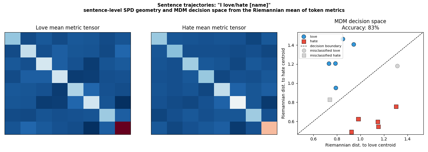
Visualise results

Two panels show (1) the Riemannian mean metric tensor per class, and (2) the MDM decision space with the Riemannian distance to each class centroid.

palette = {"love": "#3498DB", "hate": "#E84C3D"}
mdm = pipeline[-1]

all_tokens = np.vstack(x_list)
dist_love = distance(sentence_spd, mdm.covmeans_[0], metric="riemann")[:, 0]
dist_hate = distance(sentence_spd, mdm.covmeans_[1], metric="riemann")[:, 0]


fig, axes = plt.subplots(1, 3, figsize=(14, 5))
fig.suptitle(
    'Sentence trajectories: "I love/hate [name]"\n'
    "sentence-level SPD geometry and MDM decision space "
    "from the Riemannian mean of token metrics",
    fontsize=11, fontweight="bold",
)

mean_love = mean_riemann(sentence_spd[y == 0])
mean_hate = mean_riemann(sentence_spd[y == 1])
vmax = max(mean_love.max(), mean_hate.max())
vmin = min(mean_love.min(), mean_hate.min())
for ax, mat, title in zip(
    axes[:2],
    [mean_love, mean_hate],
    ["Love mean metric tensor", "Hate mean metric tensor"],
):
    im = ax.imshow(mat, cmap="RdBu_r", aspect="auto", vmin=vmin, vmax=vmax)
    ax.set_title(title)
    ax.set_xticks([])
    ax.set_yticks([])

ax = axes[2]
correct = y_pred == y
for cls, verb in enumerate(["love", "hate"]):
    mask = y == cls
    fc = [palette[verb] if ok else "lightgray" for ok in correct[mask]]
    ec = ["k" if ok else "#888888" for ok in correct[mask]]
    ax.scatter(
        dist_love[mask], dist_hate[mask],
        c=fc, edgecolors=ec,
        marker="o" if cls == 0 else "s",
        s=90, linewidths=0.6,
        label=verb,
    )
_kw = dict(linestyle="none", color="lightgray", markeredgecolor="#888888",
           markeredgewidth=0.6, markersize=9)
error_love = Line2D([], [], marker="o", label="misclassified love", **_kw)
error_hate = Line2D([], [], marker="s", label="misclassified hate", **_kw)
lims = [
    min(dist_love.min(), dist_hate.min()) * 0.95,
    max(dist_love.max(), dist_hate.max()) * 1.05,
]
ax.plot(lims, lims, "k--", lw=1, label="decision boundary")
ax.set_xlim(lims)
ax.set_ylim(lims)
ax.set_title(f"MDM decision space\nAccuracy: {correct.mean():.0%}")
ax.set_xlabel("Riemannian dist. to love centroid")
ax.set_ylabel("Riemannian dist. to hate centroid")
handles, labels = ax.get_legend_handles_labels()
ax.legend(handles=[*handles, error_love, error_hate], fontsize=8)

plt.tight_layout()

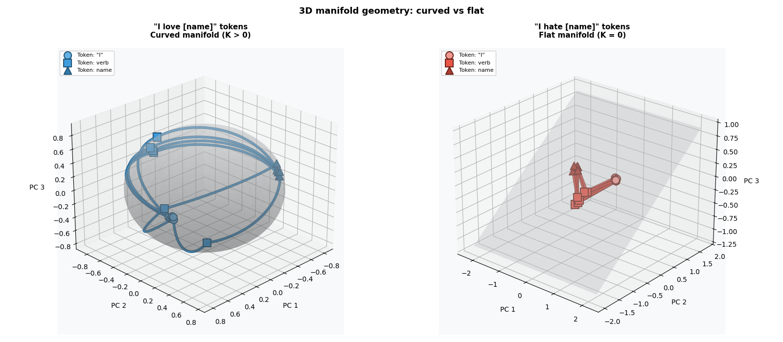
3D Manifold Visualization

This figure shows an example of how Riemannian geometry can help us with understanding Language Models: “love” and “hate” sentences trace different geometric structures. Love tokens lie on a positively curved sphere (K > 0) with geodesic arcs, while hate tokens lie on a flat plane (K = 0) with straight trajectories. This curvature difference—captured by local metric tensors enables MDM classification, thanks to treating LLMs latent space as a Riemannian manifold we can extract many geometric features that may be benefitial in understanding and classification of sentences produced by LLMs.

# Compute 3D embeddings for surface visualization
all_3d = PCA(n_components=3, random_state=0).fit_transform(all_tokens)
token_cls_3d = np.repeat(y, N_TOKENS)

# Separate love and hate tokens in 3D
love_3d = all_3d[token_cls_3d == 0]
hate_3d = all_3d[token_cls_3d == 1]

# Create new figure for 3D visualizations
fig_3d = plt.figure(figsize=(16, 7))
fig_3d.suptitle(
    "3D manifold geometry: curved vs flat",
    fontsize=13, fontweight="bold", y=0.98,
)

# Panel 1: Curved manifold (love tokens)
ax1 = fig_3d.add_subplot(1, 2, 1, projection='3d')

# Fit sphere for love tokens first
love_center = love_3d.mean(axis=0)
radius = np.mean(np.linalg.norm(love_3d - love_center, axis=1))

# Project love tokens onto sphere surface
love_3d_projected = project_to_sphere(love_3d, love_center, radius)

# Plot love tokens on sphere surface with different markers and shades
# per token type. Token order: [I, verb, name] for each sentence
token_markers = ['o', 's', '^']  # circle, square, triangle
token_labels = ['Token: "I"', 'Token: verb', 'Token: name']
token_sizes = [120, 140, 120]
token_colors = ['#5DADE2', '#3498DB', '#2874A6']  # light, medium, dark blue

scatter_token_groups(
    ax1, love_3d_projected, token_colors, '#1B4F72',
    token_markers, token_labels, token_sizes,
)

# Draw love sentence trajectories as geodesics on sphere surface
traj_3d = all_3d.reshape(-1, N_TOKENS, 3)
for traj in traj_3d[y == 0]:
    # Project trajectory points onto sphere
    traj_proj = project_to_sphere(traj, love_center, radius)

    # Draw geodesics (great circles) between consecutive points
    for i in range(len(traj_proj) - 1):
        p1 = traj_proj[i] - love_center
        p2 = traj_proj[i + 1] - love_center

        # Normalize to unit sphere
        p1_norm = p1 / np.linalg.norm(p1)
        p2_norm = p2 / np.linalg.norm(p2)

        # Calculate angle between points
        cos_angle = np.clip(np.dot(p1_norm, p2_norm), -1.0, 1.0)
        angle = np.arccos(cos_angle)

        # Generate points along the geodesic (great circle arc)
        n_points = max(20, int(angle * 50))

        # Slerp (Spherical Linear Interpolation) for geodesic
        if angle > 1e-6:  # Avoid division by zero
            t = np.linspace(0, 1, n_points)[:, None]
            geodesic = (
                np.sin((1 - t) * angle) * p1_norm
                + np.sin(t * angle) * p2_norm
            ) / np.sin(angle)
            geodesic = love_center + radius * geodesic
            plot_outlined_3d(ax1, geodesic, palette["love"])

# Plot sphere surface in grey with stretched z-dimension
u = np.linspace(0, 2 * np.pi, 40)
v = np.linspace(0, np.pi, 40)
x_sphere = radius * np.outer(np.cos(u), np.sin(v)) + love_center[0]
y_sphere = radius * np.outer(np.sin(u), np.sin(v)) + love_center[1]
z_sphere = radius * np.outer(np.ones(np.size(u)), np.cos(v)) + love_center[2]

ax1.plot_surface(
    x_sphere, y_sphere, z_sphere,
    color='#D5D8DC', alpha=0.3, edgecolor="none",
    antialiased=True, shade=True,
)

# Add wireframe for better depth perception
ax1.plot_wireframe(
    x_sphere, y_sphere, z_sphere, color='#85929E', alpha=0.15,
    linewidth=0.3, rstride=4, cstride=4,
)

ax1.set_title(
    '"I love [name]" tokens\nCurved manifold (K > 0)',
    fontsize=11, fontweight="bold", pad=15,
)
ax1.set_xlabel("PC 1", fontsize=10, labelpad=10)
ax1.set_ylabel("PC 2", fontsize=10, labelpad=10)
ax1.set_zlabel("PC 3", fontsize=10, labelpad=10)
ax1.view_init(elev=25, azim=45)
ax1.grid(True, alpha=0.3)
ax1.set_facecolor("#f8f9fa")
ax1.legend(loc='upper left', fontsize=8, framealpha=0.9)

# Panel 2: Flat manifold (hate tokens)
ax2 = fig_3d.add_subplot(1, 2, 2, projection='3d')

# Different shades of red for each token type
token_colors_hate = ['#F1948A', '#E74C3C', '#A93226']

# Plot hate tokens with different markers and shades per token type
scatter_token_groups(
    ax2, hate_3d, token_colors_hate, '#641E16',
    token_markers, token_labels, token_sizes,
)

# Draw hate sentence trajectories in 3D with outlines
for traj in traj_3d[y == 1]:
    plot_outlined_3d(ax2, traj, palette["hate"], outline="#641E16")

# Fit and plot plane surface for hate tokens
if len(hate_3d) > 2:
    hate_center = hate_3d.mean(axis=0)
    hate_centered = hate_3d - hate_center
    _, _, Vt = np.linalg.svd(hate_centered)

    # Use first two principal components to define plane
    normal = Vt[2]

    # Create extended plane surface
    extent = 1.5  # Extend plane beyond data points
    xlim = [hate_3d[:, 0].min() - extent, hate_3d[:, 0].max() + extent]
    ylim = [hate_3d[:, 1].min() - extent, hate_3d[:, 1].max() + extent]
    xx, yy = np.meshgrid(
        np.linspace(xlim[0], xlim[1], 30),
        np.linspace(ylim[0], ylim[1], 30),
    )

    # Calculate z for the plane
    d = -hate_center.dot(normal)
    zz = (-normal[0] * xx - normal[1] * yy - d) / (normal[2] + 1e-10)

    ax2.plot_surface(
        xx, yy, zz,
        color='#D5D8DC', alpha=0.35, edgecolor="none",
        antialiased=True, shade=True,
    )

ax2.set_title(
    '"I hate [name]" tokens\nFlat manifold (K = 0)',
    fontsize=11, fontweight="bold", pad=15,
)
ax2.set_xlabel("PC 1", fontsize=10, labelpad=10)
ax2.set_ylabel("PC 2", fontsize=10, labelpad=10)
ax2.set_zlabel("PC 3", fontsize=10, labelpad=10)
ax2.grid(True, alpha=0.3)
ax2.set_facecolor("#f8f9fa")
ax2.legend(loc='upper left', fontsize=8, framealpha=0.9)
ax2.view_init(elev=25, azim=-50)

plt.tight_layout()
plt.show()

0), "I hate [name]" tokens Flat manifold (K = 0)" class = "sphx-glr-single-img"/>

References

[1] (1,2)

Poincaré GloVe: Hyperbolic Word Embeddings A. Tifrea, G. Bécigneul, and O.-E. Ganea, ICLR, 2019.

[2] (1,2)

Emergence of a High-Dimensional Abstraction Phase in Language Transformers E. Cheng, D. Doimo, C. Kervadec, I. Macocco, J. Yu, A. Laio, and M. Baroni, ICLR, 2025.