Mean and median comparison

A comparison between Euclidean and Riemannian means [1], and Euclidean and Riemannian geometric medians [2], on low-dimensional synthetic datasets.

# Authors: Quentin Barthélemy
#
# License: BSD (3-clause)

import numpy as np
import matplotlib.pyplot as plt

from sklearn.datasets import make_blobs
from pyriemann.datasets import make_outliers
from pyriemann.utils import mean_euclid, mean_riemann
from pyriemann.utils import median_euclid, median_riemann
from pyriemann.clustering import Potato

rs = np.random.RandomState(17)

Data in vector space

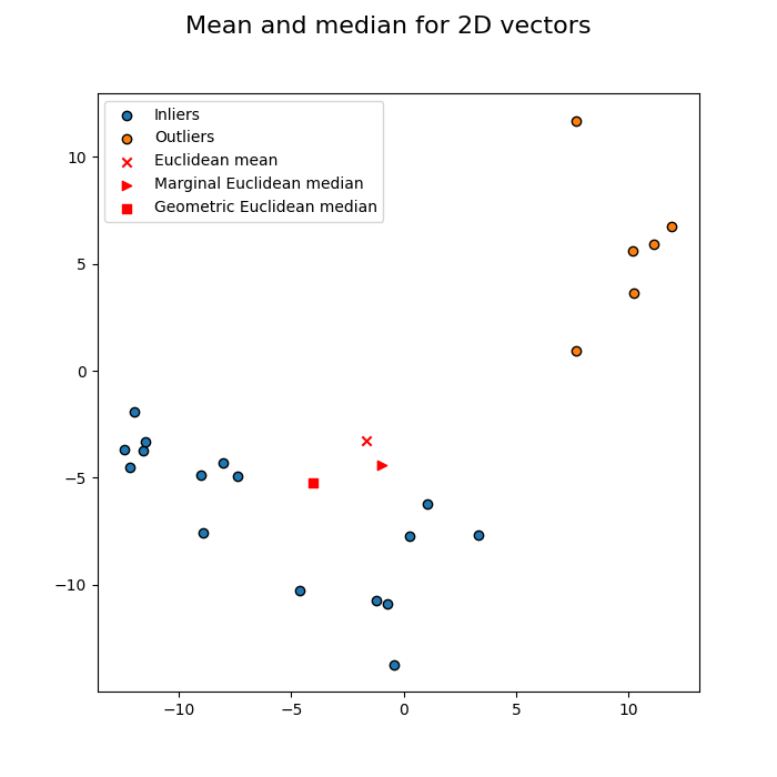
Dataset of 2D vectors, reproducing Fig 1 of reference [2].

Notice how the few outliers at the top right of the picture have forced the mean away from the points, whereas the geometric median remains centrally located.

X, y = make_blobs(
    n_samples=[7, 9, 6],
    n_features=2,
    centers=np.array([[-1, -10], [-10, -4], [10, 5]]),
    cluster_std=[2, 2, 2],
    random_state=rs
)
is_inlier = (y <= 1)

C_mean = mean_euclid(X[..., np.newaxis])
C_mmed = np.median(X, axis=0)
C_gmed = median_euclid(X[..., np.newaxis])

fig, ax = plt.subplots(figsize=(7, 7))
fig.suptitle("Mean and median for 2D vectors", fontsize=16)
ax.scatter(X[is_inlier, 0], X[is_inlier, 1], c='C0', edgecolors="k",
           label='Inliers')
ax.scatter(X[~is_inlier, 0], X[~is_inlier, 1], c='C1', edgecolors="k",
           label='Outliers')
ax.scatter(C_mean[0], C_mean[1], c='r', marker="x", label='Euclidean mean')
ax.scatter(C_mmed[0], C_mmed[1], c='r', marker=">",
           label='Marginal Euclidean median')
ax.scatter(C_gmed[0], C_gmed[1], c='r', marker="s",
           label='Geometric Euclidean median')
ax.legend(loc='upper left')
plt.show()

Data in manifold of SPD matrices

Dataset of 2x2 SPD matrices.

A dynamic display is required if you want to rotate or zoom the 3D figure. This 3D plot can be tricky to interpret. 2x2 SPD matrices can be viewed as spatial coordinates contained in a hyper-cone [3]. In Euclidean geometry, null matrix is the center of space. In Riemannian geometry, identity matrix is the center of the unbounded and non-linear manifold [3]: due to log(.)^2 in the affine-invariant distance, an eigenvalue of 10 contributes to the distance from the identity as much as an eigenvalue 0.1.

n_channels, n_inliers, n_outliers = 2, 16, 6

Cin = 0.2 * np.eye(n_channels)
Xin = make_outliers(n_inliers, Cin, 0.5, outlier_coeff=1, random_state=rs)
Xout = make_outliers(
    n_outliers, 4 * np.eye(n_channels), 0.5, outlier_coeff=1, random_state=rs)
X = np.concatenate([Xin, Xout])

C_emean = mean_euclid(X)
C_rmean = mean_riemann(X)
C_emed = median_euclid(X)
C_rmed = median_riemann(X)

fig2 = plt.figure(figsize=(7, 7))
fig2.suptitle("Means and medians for 2x2 SPD matrices", fontsize=16)
ax2 = plt.subplot(111, projection='3d')
ax2.scatter(1, 0, 1, c="k", marker="+", s=50, label='Identity')
ax2.scatter(Xin[:, 0, 0], Xin[:, 0, 1], Xin[:, 1, 1], c="C0", edgecolors="k",
            label='Inliers')
ax2.scatter(Xout[:, 0, 0], Xout[:, 0, 1], Xout[:, 1, 1], c="C1",
            edgecolors="k", label='Outliers')
ax2.scatter(C_emean[0, 0], C_emean[0, 1], C_emean[1, 1], c="r", marker="x",
            label='Euclidean mean')
ax2.scatter(C_rmean[0, 0], C_rmean[0, 1], C_rmean[1, 1], c="m", marker="x",
            label='Riemannian mean')
ax2.scatter(C_emed[0, 0], C_emed[0, 1], C_emed[1, 1], c="r", marker="s",
            label='Euclidean median')
ax2.scatter(C_rmed[0, 0], C_rmed[0, 1], C_rmed[1, 1], c="m", marker="s",
            label='Riemannian median')
ax2.legend(loc='center left', bbox_to_anchor=(0.7, 0.6))
plt.show()

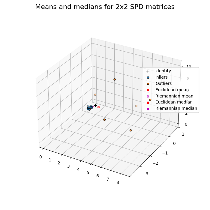
Photo finish

Specific zoom on means and medians.

Surprise guest: Riemannian potato is fitted with an offline iterative outlier removal, providing a robust mean [4].

C_rp = Potato(metric='riemann', threshold=1.5).fit(X).covmean_

fig3 = plt.figure(figsize=(7, 7))
fig3.suptitle("Means and medians for 2x2 SPD matrices\nZoom", fontsize=16)
ax3 = plt.subplot(111, projection='3d')
ax3.scatter(1, 0, 1, c="k", marker="+", s=50, label='Identity')
ax3.scatter(Cin[0, 0], Cin[0, 1], Cin[1, 1], c="C0", edgecolors="k", s=50,
            label='Center of inliers')
ax3.scatter(C_emean[0, 0], C_emean[0, 1], C_emean[1, 1], c="r", marker="x",
            label='Euclidean mean')
ax3.scatter(C_rmean[0, 0], C_rmean[0, 1], C_rmean[1, 1], c="m", marker="x",
            label='Riemannian mean')
ax3.scatter(C_emed[0, 0], C_emed[0, 1], C_emed[1, 1], c="r", marker="s",
            label='Euclidean median')
ax3.scatter(C_rmed[0, 0], C_rmed[0, 1], C_rmed[1, 1], c="m", marker="s",
            label='Riemannian median')
ax3.scatter(C_rp[0, 0], C_rp[0, 1], C_rp[1, 1], c="chartreuse", marker="*",
            s=40, label='Center of\nRiemannian potato')
ax3.legend(loc='center left', bbox_to_anchor=(0.7, 0.5))
plt.show()

References

[1]

Review of Riemannian distances and divergences, applied to SSVEP-based BCI S. Chevallier, E. K. Kalunga, Q. Barthélemy, E. Monacelli. Neuroinformatics, Springer, 2021, 19 (1), pp.93-106

[2] (1,2)

The geometric median on Riemannian manifolds with application to robust atlas estimation PT. Fletcher, S. Venkatasubramanian S and S. Joshi. NeuroImage, 2009, 45(1), S143-S152

[3] (1,2)

EEG source analysis M. Congedo. HdR, 2013, Chap IX

[4]

The Riemannian Potato Field: A Tool for Online Signal Quality Index of EEG Q. Barthélemy, L. Mayaud, D. Ojeda, and M. Congedo. IEEE Transactions on Neural Systems and Rehabilitation Engineering, 2019, 27 (2), pp.244-255