Classifier comparison

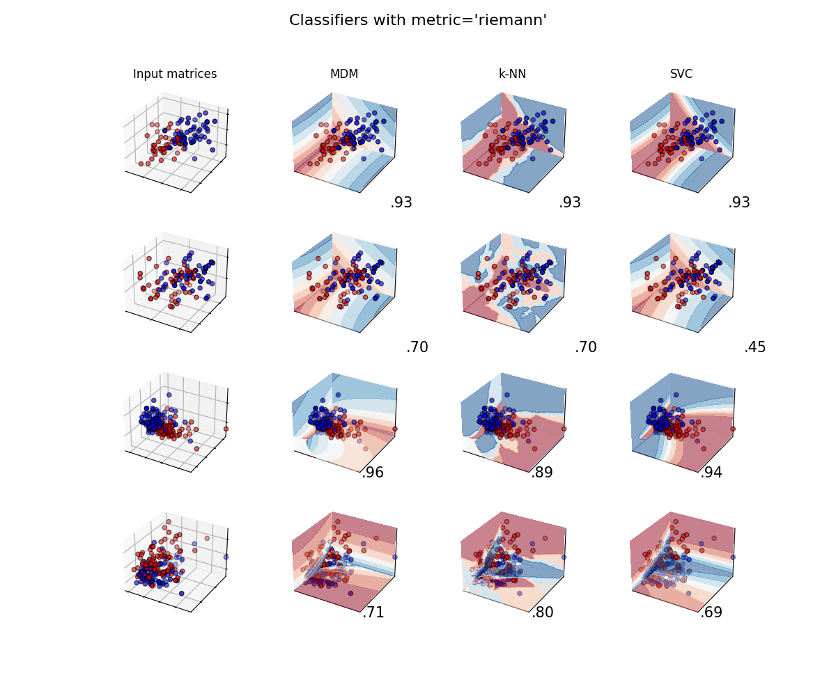
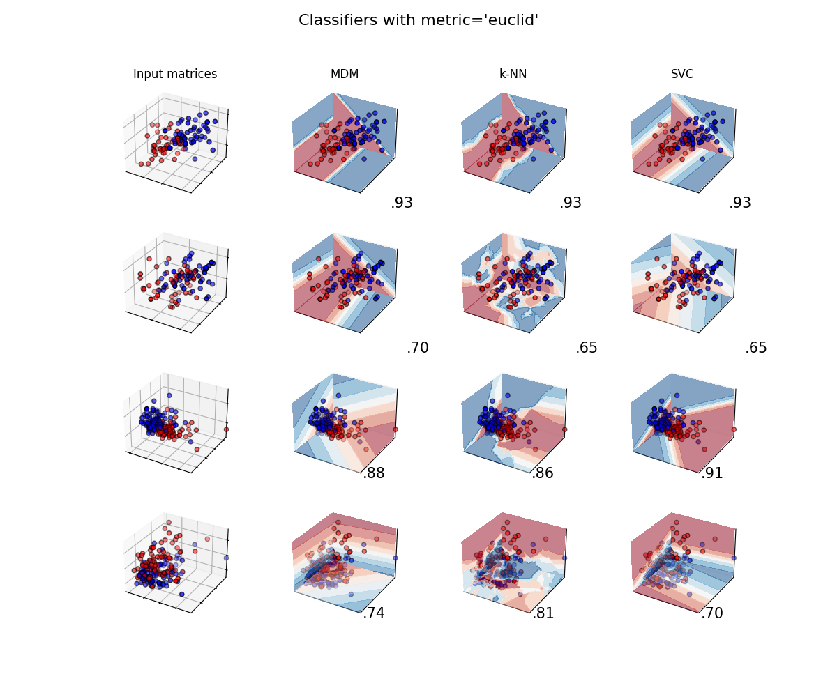
A comparison of several classifiers on low-dimensional synthetic datasets, adapted to SPD matrices from [1]. The point of this example is to illustrate the nature of decision boundaries of different classifiers, used with different metrics [2]. This should be taken with a grain of salt, as the intuition conveyed by these examples does not necessarily carry over to real datasets.

The 3D plots show training matrices in solid colors and testing matrices semi-transparent. The lower right shows the classification accuracy on the test set.

# Authors: Quentin Barthélemy
#
# License: BSD (3-clause)

from functools import partial
from time import time

import numpy as np
import matplotlib.pyplot as plt
from matplotlib.colors import ListedColormap
from sklearn.model_selection import train_test_split

from pyriemann.datasets import make_matrices, make_gaussian_blobs
from pyriemann.classification import (
    MDM,
    KNearestNeighbor,
    SVC,
    MeanField,
)

@partial(np.vectorize, excluded=['clf'])
def get_proba(cov_00, cov_01, cov_11, clf):
    cov = np.array([[cov_00, cov_01], [cov_01, cov_11]])
    with np.testing.suppress_warnings() as sup:
        sup.filter(RuntimeWarning)
        return clf.predict_proba(cov[np.newaxis, ...])[0, 1]


def plot_classifiers(metric):
    figure = plt.figure(figsize=(12, 10))
    figure.suptitle(f"Compare classifiers with metric='{metric}'", fontsize=16)
    i = 1

    # iterate over datasets
    for ds_cnt, (X, y) in enumerate(datasets):
        # split dataset into training and test part
        X_train, X_test, y_train, y_test = train_test_split(
            X, y, test_size=0.4, random_state=42
        )

        x_min, x_max = X[:, 0, 0].min(), X[:, 0, 0].max()
        y_min, y_max = X[:, 0, 1].min(), X[:, 0, 1].max()
        z_min, z_max = X[:, 1, 1].min(), X[:, 1, 1].max()

        # just plot the dataset first
        ax = plt.subplot(n_datasets, n_classifs + 1, i, projection='3d')
        if ds_cnt == 0:
            ax.set_title("Input data")
        # Plot the training points
        ax.scatter(
            X_train[:, 0, 0],
            X_train[:, 0, 1],
            X_train[:, 1, 1],
            c=y_train,
            cmap=cm_bright,
            edgecolors="k"
        )
        # Plot the testing points
        ax.scatter(
            X_test[:, 0, 0],
            X_test[:, 0, 1],
            X_test[:, 1, 1],
            c=y_test,
            cmap=cm_bright,
            alpha=0.6,
            edgecolors="k"
        )
        ax.set_xlim(x_min, x_max)
        ax.set_ylim(y_min, y_max)
        ax.set_zlim(z_min, z_max)
        ax.set_xticklabels(())
        ax.set_yticklabels(())
        ax.set_zticklabels(())
        i += 1

        rx = np.arange(x_min, x_max, (x_max - x_min) / 50)
        ry = np.arange(y_min, y_max, (y_max - y_min) / 50)
        rz = np.arange(z_min, z_max, (z_max - z_min) / 50)

        print(f"Dataset n°{ds_cnt+1}")

        # iterate over classifiers
        for name, clf in zip(names, classifiers):
            ax = plt.subplot(n_datasets, n_classifs + 1, i, projection='3d')

            clf.set_params(**{'metric': metric})
            t0 = time()
            clf.fit(X_train, y_train)
            t1 = time() - t0

            t0 = time()
            score = clf.score(X_test, y_test)
            t2 = time() - t0

            print(
                f" {name}:\n  training time={t1:.5f}\n  test time    ={t2:.5f}"
            )

            # Plot the decision boundaries for horizontal 2D planes going
            # through the mean value of the third coordinates
            xx, yy = np.meshgrid(rx, ry)
            zz = get_proba(xx, yy, X[:, 1, 1].mean()*np.ones_like(xx), clf=clf)
            zz = np.ma.masked_where(~np.isfinite(zz), zz)
            ax.contourf(xx, yy, zz, zdir='z', offset=z_min, cmap=cm, alpha=0.5)

            xx, zz = np.meshgrid(rx, rz)
            yy = get_proba(xx, X[:, 0, 1].mean()*np.ones_like(xx), zz, clf=clf)
            yy = np.ma.masked_where(~np.isfinite(yy), yy)
            ax.contourf(xx, yy, zz, zdir='y', offset=y_max, cmap=cm, alpha=0.5)

            yy, zz = np.meshgrid(ry, rz)
            xx = get_proba(X[:, 0, 0].mean()*np.ones_like(yy), yy, zz, clf=clf)
            xx = np.ma.masked_where(~np.isfinite(xx), xx)
            ax.contourf(xx, yy, zz, zdir='x', offset=x_min, cmap=cm, alpha=0.5)

            # Plot the training points
            ax.scatter(
                X_train[:, 0, 0],
                X_train[:, 0, 1],
                X_train[:, 1, 1],
                c=y_train,
                cmap=cm_bright,
                edgecolors="k"
            )
            # Plot the testing points
            ax.scatter(
                X_test[:, 0, 0],
                X_test[:, 0, 1],
                X_test[:, 1, 1],
                c=y_test,
                cmap=cm_bright,
                edgecolors="k",
                alpha=0.6
            )

            if ds_cnt == 0:
                ax.set_title(name)
            ax.text(
                1.3 * x_max,
                y_min,
                z_min,
                ("%.2f" % score).lstrip("0"),
                size=15,
                horizontalalignment="right",
                verticalalignment="bottom"
            )
            ax.set_xlim(x_min, x_max)
            ax.set_ylim(y_min, y_max)
            ax.set_zlim(z_min, z_max)
            ax.set_xticks(())
            ax.set_yticks(())
            ax.set_zticks(())

            i += 1

    plt.show()

Classifiers and Datasets

names = [
    "MDM",
    "k-NN",
    "SVC",
    "MeanField",
]
classifiers = [
    MDM(),
    KNearestNeighbor(n_neighbors=3),
    SVC(probability=True),
    MeanField(power_list=[-1, 0, 1]),
]
n_classifs = len(classifiers)

rs = np.random.RandomState(2022)
n_matrices, n_channels = 50, 2
y = np.concatenate([np.zeros(n_matrices), np.ones(n_matrices)])

datasets = [
    (
        np.concatenate([
            make_matrices(
                n_matrices, n_channels, "spd", rs, evals_low=10, evals_high=14
            ),
            make_matrices(
                n_matrices, n_channels, "spd", rs, evals_low=13, evals_high=17
            )
        ]),
        y
    ),
    (
        np.concatenate([
            make_matrices(
                n_matrices, n_channels, "spd", rs, evals_low=10, evals_high=14
            ),
            make_matrices(
                n_matrices, n_channels, "spd", rs, evals_low=11, evals_high=15
            )
        ]),
        y
    ),
    make_gaussian_blobs(
        2*n_matrices, n_channels, random_state=rs, class_sep=1., class_disp=.5,
        n_jobs=4
    ),
    make_gaussian_blobs(
        2*n_matrices, n_channels, random_state=rs, class_sep=.5, class_disp=.5,
        n_jobs=4
    )
]
n_datasets = len(datasets)

cm = plt.cm.RdBu
cm_bright = ListedColormap(["#FF0000", "#0000FF"])

Classifiers with Riemannian metric

plot_classifiers("riemann")

Dataset n°1
 MDM:
  training time=0.00293
  test time    =0.00681
 k-NN:
  training time=0.00006
  test time    =0.13814
 SVC:
  training time=0.00460
  test time    =0.00197
 MeanField:
  training time=0.00338
  test time    =0.02028
Dataset n°2
 MDM:
  training time=0.00281
  test time    =0.00662
 k-NN:
  training time=0.00006
  test time    =0.13819
 SVC:
  training time=0.00446
  test time    =0.00192
 MeanField:
  training time=0.00619
  test time    =0.01830
Dataset n°3
 MDM:
  training time=0.00596
  test time    =0.01214
 k-NN:
  training time=0.00006
  test time    =0.39111
 SVC:
  training time=0.00737
  test time    =0.00211
 MeanField:
  training time=0.00661
  test time    =0.03868
Dataset n°4
 MDM:
  training time=0.00590
  test time    =0.01205
 k-NN:
  training time=0.00006
  test time    =0.39407
 SVC:
  training time=0.00764
  test time    =0.00225
 MeanField:
  training time=0.00657
  test time    =0.03866

Classifiers with Log-Euclidean metric

plot_classifiers("logeuclid")

Dataset n°1
 MDM:
  training time=0.00084
  test time    =0.00980
 k-NN:
  training time=0.00006
  test time    =0.18602
 SVC:
  training time=0.00279
  test time    =0.00174
 MeanField:
  training time=0.00344
  test time    =0.03058
Dataset n°2
 MDM:
  training time=0.00086
  test time    =0.00975
 k-NN:
  training time=0.00006
  test time    =0.18779
 SVC:
  training time=0.00283
  test time    =0.00174
 MeanField:
  training time=0.00343
  test time    =0.03062
Dataset n°3
 MDM:
  training time=0.00094
  test time    =0.01847
 k-NN:
  training time=0.00006
  test time    =0.59480
 SVC:
  training time=0.00333
  test time    =0.00190
 MeanField:
  training time=0.00667
  test time    =0.05992
Dataset n°4
 MDM:
  training time=0.00098
  test time    =0.01835
 k-NN:
  training time=0.00005
  test time    =0.63659
 SVC:
  training time=0.00416
  test time    =0.00193
 MeanField:
  training time=0.00657
  test time    =0.05915

Classifiers with Euclidean metric

plot_classifiers("euclid")

Dataset n°1
 MDM:
  training time=0.00039
  test time    =0.00249
 k-NN:
  training time=0.00006
  test time    =0.04487
 SVC:
  training time=0.00191
  test time    =0.00137
 MeanField:
  training time=0.00343
  test time    =0.00774
Dataset n°2
 MDM:
  training time=0.00040
  test time    =0.00249
 k-NN:
  training time=0.00006
  test time    =0.04506
 SVC:
  training time=0.00262
  test time    =0.00132
 MeanField:
  training time=0.00342
  test time    =0.00767
Dataset n°3
 MDM:
  training time=0.00043
  test time    =0.00381
 k-NN:
  training time=0.00006
  test time    =0.13714
 SVC:
  training time=0.00356
  test time    =0.00137
 MeanField:
  training time=0.00654
  test time    =0.01371
Dataset n°4
 MDM:
  training time=0.00040
  test time    =0.00383
 k-NN:
  training time=0.00006
  test time    =0.13670
 SVC:
  training time=0.00321
  test time    =0.00141
 MeanField:
  training time=0.00675
  test time    =0.01398

References

[1]

https://scikit-learn.org/stable/auto_examples/classification/plot_classifier_comparison.html # noqa

[2]

Review of Riemannian distances and divergences, applied to SSVEP-based BCI S. Chevallier, E. K. Kalunga, Q. Barthélemy, E. Monacelli. Neuroinformatics, Springer, 2021, 19 (1), pp.93-106