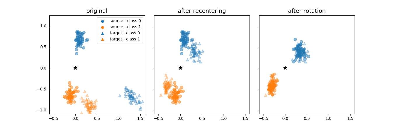
Data transformations in the Riemannian Procrustes Analysis

Use the SpectralEmbedding module to plot in 2D the transformations on the matrices from source and target domains when applying the Riemannian Procrustes Analysis [1] to match their statistics.

import matplotlib.pyplot as plt
import numpy as np

from pyriemann.datasets.simulated import make_classification_transfer
from pyriemann.embedding import SpectralEmbedding
from pyriemann.transfer import decode_domains, TLCenter, TLRotate

# Fix seed for reproducible results
seed = 66

# create source and target datasets
n_matrices = 50
X_enc, y_enc = make_classification_transfer(
    n_matrices=n_matrices,
    class_sep=2.0,
    class_disp=0.25,
    domain_sep=2.0,
    theta=np.pi/4,
    random_state=seed
)

# generate dataset
X_org, y, domain = decode_domains(X_enc, y_enc)

# instantiate object for doing spectral embeddings
emb = SpectralEmbedding(n_components=2, metric="riemann")

# create dict to store the embedding after each step of RPA
embedded_points = {}

# embed the original source and target datasets
points = np.concatenate([X_org, np.eye(2)[None, :, :]])  # stack the identity
embedded_points["origin"] = emb.fit_transform(points)

# embed the source and target datasets after recentering
rct = TLCenter(target_domain="target_domain")
X_rct = rct.fit_transform(X_org, y_enc)
points = np.concatenate([X_rct, np.eye(2)[None, :, :]])  # stack the identity
embedded_points["rct"] = emb.fit_transform(points)

# embed the source and target datasets after recentering
rot = TLRotate(target_domain="target_domain", metric="riemann")
X_rot = rot.fit_transform(X_rct, y_enc)

points = np.concatenate([X_org, X_rct, X_rot, np.eye(2)[None, :, :]])
S = emb.fit_transform(points)
S = S - S[-1]
embedded_points["origin"] = S[:4*n_matrices]
embedded_points["rct"] = S[4*n_matrices:8*n_matrices]
embedded_points["rot"] = S[8*n_matrices:-1]

Plot the results, reproducing the Figure 1 of [1].

fig, ax = plt.subplots(figsize=(13.5, 4.4), ncols=3, sharey=True)
plt.subplots_adjust(wspace=0.10)
steps = ["origin", "rct", "rot"]
titles = ["original", "after recentering", "after rotation"]
for axi, step, title in zip(ax, steps, titles):
    S_step = embedded_points[step]
    S_source = S_step[domain == "source_domain"]
    y_source = y[domain == "source_domain"]
    S_target = S_step[domain == "target_domain"]
    y_target = y[domain == "target_domain"]
    axi.scatter(
        S_source[y_source == "1"][:, 0],
        S_source[y_source == "1"][:, 1],
        c="C0", s=50, alpha=0.50,
    )
    axi.scatter(
        S_source[y_source == "2"][:, 0],
        S_source[y_source == "2"][:, 1],
        c="C1", s=50, alpha=0.50,
    )
    axi.scatter(
        S_target[y_target == "1"][:, 0],
        S_target[y_target == "1"][:, 1],
        c="C0", s=50, alpha=0.30, marker="^",
    )
    axi.scatter(
        S_target[y_target == "2"][:, 0],
        S_target[y_target == "2"][:, 1],
        c="C1", s=50, alpha=0.30, marker="^",
    )
    axi.scatter(S[-1, 0], S[-1, 1], c="k", s=80, marker="*")
    axi.set_xlim(-0.60, +1.60)
    axi.set_ylim(-1.10, +1.25)
    axi.set_xticks([-0.5, 0.0, 0.5, 1.0, 1.5])
    axi.set_yticks([-1.0, -0.5, 0.0, 0.5, 1.0])
    axi.set_title(title, fontsize=14)
ax[0].scatter([], [], c="C0", label="source - class 0")
ax[0].scatter([], [], c="C1", label="source - class 1")
ax[0].scatter([], [], marker="^", c="C0", label="target - class 0")
ax[0].scatter([], [], marker="^", c="C1", label="target - class 1")
ax[0].legend(loc="upper right")
plt.show()

References

[1] (1,2)

Riemannian Procrustes analysis: transfer learning for brain-computer interfaces PLC Rodrigues et al, IEEE Transactions on Biomedical Engineering, vol. 66, no. 8, pp. 2390-2401, December, 2018