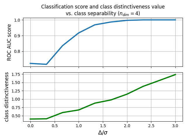
Classification accuracy vs class distinctiveness vs class separability

Generate several datasets containing data points from two-classes. Each class is generated with a Riemannian Gaussian distribution centered at the class mean and with the same dispersion sigma. The distance between the class means is parametrized by Delta, which we make vary between zero and 5*sigma. We illustrate how the accuracy of the MDM classifier and the value of the class distinctiveness [1] vary when Delta increases.

# Authors: Pedro Rodrigues <pedro.rodrigues@melix.org>
#          Maria Sayu Yamamoto <maria-sayu.yamamoto@universite-paris-saclay.fr>
#
# License: BSD (3-clause)

import numpy as np
import matplotlib.pyplot as plt
from sklearn.model_selection import cross_val_score, StratifiedKFold

from pyriemann.classification import MDM
from pyriemann.datasets import make_gaussian_blobs
from pyriemann.classification import class_distinctiveness

Set general parameters for the illustrations

n_matrices = 100  # how many matrices to sample on each class
n_dim = 4  # dimensionality of the data points
sigma = 1.0  # dispersion of the Gaussian distributions
random_state = 42  # ensure reproducibility

Loop over different levels of separability between the classes

scores_array = []
class_dis_array = []
deltas_array = np.linspace(0, 3*sigma, 10)

for delta in deltas_array:
    # generate data points for a classification problem
    X, y = make_gaussian_blobs(n_matrices=n_matrices,
                               n_dim=n_dim,
                               class_sep=delta,
                               class_disp=sigma,
                               random_state=random_state,
                               n_jobs=4)

    # measure class distinctiveness of training data for each split
    skf = StratifiedKFold(n_splits=5)
    all_class_dis = []
    for train_ind, _ in skf.split(X, y):
        class_dis = class_distinctiveness(X[train_ind], y[train_ind],
                                          exponent=1, metric='riemann',
                                          return_num_denom=False)
        all_class_dis.append(class_dis)

    # average class distinctiveness across splits
    mean_class_dis = np.mean(all_class_dis)
    class_dis_array.append(mean_class_dis)

    # Now let's train a MDM classifier and measure its performance
    clf = MDM()

    # get the classification score for this setup
    scores_array.append(
        cross_val_score(clf, X, y, cv=skf, scoring='roc_auc').mean())

scores_array = np.array(scores_array)
class_dis_array = np.array(class_dis_array)

Plot the results

fig, (ax1, ax2) = plt.subplots(sharex=True, nrows=2)

ax1.plot(deltas_array, scores_array, lw=3.0, label=r'ROC AUC score')
ax2.plot(deltas_array, class_dis_array, lw=3.0, color='g',
         label='Class Distinctiveness')

ax2.set_xlabel(r'$\Delta/\sigma$', fontsize=14)
ax1.set_ylabel(r'ROC AUC score', fontsize=12)
ax2.set_ylabel(r'class distinctiveness', fontsize=12)
ax1.set_title('Classification score and class distinctiveness value\n'
              r'vs. class separability ($n_{dim} = 4$)',
              fontsize=12)

ax1.grid(True)
ax2.grid(True)
fig.tight_layout()
plt.show()

References

[1]

Class-distinctiveness-based frequency band selection on the Riemannian manifold for oscillatory activity-based BCIs: preliminary results M. S. Yamamoto, F. Lotte, F. Yger, and S. Chevallier. 44th Annual International Conference of the IEEE Engineering in Medicine & Biology Society (EMBC2022), 2022.