Metric comparison¶

A comparison of the usual metrics used to process SPD matrices, computed mainly for 2x2 matrices to display intuitive visualizations.

# Authors: Quentin Barthélemy
#
# License: BSD (3-clause)

import matplotlib.pyplot as plt
from matplotlib import colors
from matplotlib.patches import Ellipse
import numpy as np

from pyriemann.datasets import make_gaussian_blobs
from pyriemann.geometry.geodesic import (
    geodesic_euclid,
    geodesic_logeuclid,
    geodesic_riemann,
)
from pyriemann.geometry.mean import gmean

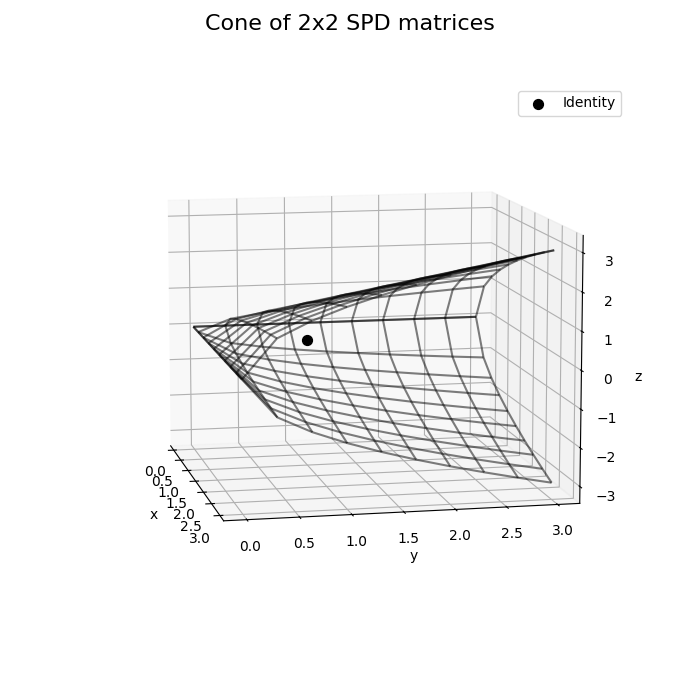
Cone of SPD matrices¶

2X2 SPD matrices [[x, z], [z, y]] are characterized by x > 0, y > 0 and a positive determinant, ie xy - z^2 > 0.

Then, matrices can be represented as points in R^3 and the constraints can be plotted as an open convex second-order cone, whose boundaries are defined by z = +/- sqrt(xy).

This figure reproduces Fig 3 of reference [1].

x = np.linspace(0, 3, 10)
y = np.linspace(0, 3, 10)
X, Y = np.meshgrid(x, y)
Z = np.sqrt(X * Y)

fig = plt.figure(figsize=(7, 7))
fig.suptitle("Cone of 2x2 SPD matrices", fontsize=16)
ax = plt.subplot(111, projection="3d")
ax.set(xlabel="x", ylabel="y", zlabel="z")
ax.plot_wireframe(X, Y, Z, color="k", alpha=0.5)
ax.plot_wireframe(X, Y, -Z, color="k", alpha=0.5)
ax.scatter(1, 1, 0, c="k", marker="o", s=50, label="Identity")
ax.legend()
ax.view_init(elev=10, azim=-12)
plt.show()

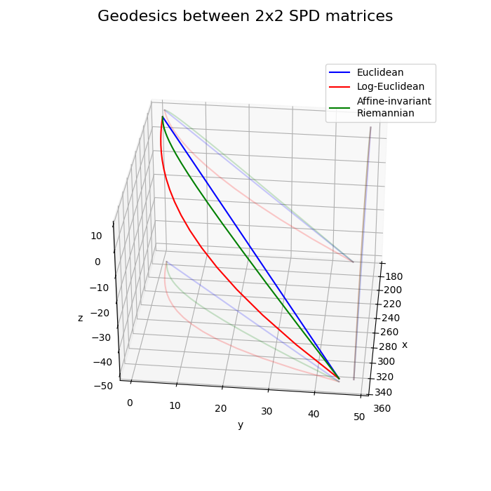
Geodesics¶

Take matrices away from identity to reinforce differences between log-Euclidean and affine-invariant Riemannian geodesics

A = np.array([[350, -50], [-50, 45]])
B = np.array([[200, 10], [10, 1]])

alphas = np.linspace(0, 1, 20)
Ge = np.array([geodesic_euclid(A, B, alpha) for alpha in alphas])
Gle = np.array([geodesic_logeuclid(A, B, alpha) for alpha in alphas])
Gr = np.array([geodesic_riemann(A, B, alpha) for alpha in alphas])

fig = plt.figure(figsize=(7, 7))
fig.suptitle("Geodesics between 2x2 SPD matrices", fontsize=16)
ax = plt.subplot(111, projection="3d")
ax.set(xlabel="x", ylabel="y", zlabel="z")
ax.plot(Ge[:, 0, 0], Ge[:, 1, 1], Ge[:, 0, 1], c="b", label="Euclidean")
ax.plot(Gle[:, 0, 0], Gle[:, 1, 1], Gle[:, 0, 1], c="r", label="Log-Euclidean")
ax.plot(Gr[:, 0, 0], Gr[:, 1, 1], Gr[:, 0, 1], c="g",
        label="Affine-invariant\nRiemannian")
xlim, ylim, zlim = ax.get_xlim()[0], ax.get_ylim()[-1], ax.get_zlim()[0]
for G, c in zip([Ge, Gle, Gr], ["b", "r", "g"]):
    ax.plot(G[:, 0, 0], G[:, 1, 1], zs=zlim, zdir="z", c=c, alpha=0.2)
    ax.plot(G[:, 0, 0], G[:, 0, 1], zs=ylim, zdir="y", c=c, alpha=0.2)
    ax.plot(G[:, 1, 1], G[:, 0, 1], zs=xlim, zdir="x", c=c, alpha=0.2)
ax.legend()
ax.view_init(elev=32, azim=6)
plt.show()

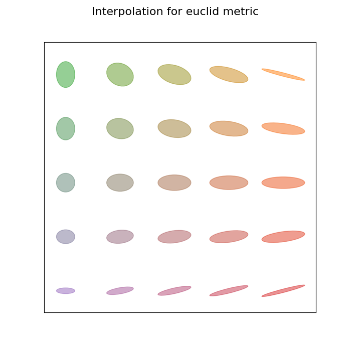
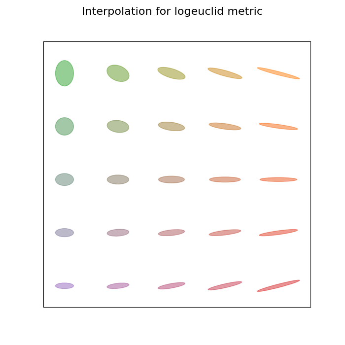
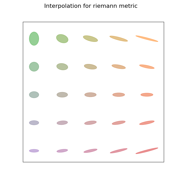
Interpolation¶

Bilinear interpolation of four SPD matrices. The “swelling effect” is clearly visible in the Euclidean case: the volume of associated ellipsoids is parabolically interpolated and reaches a maximum between the two extremities.

These figures reproduce Fig 4.2 of reference [2].

X = np.array([
    [[0.5, 0], [0, 0.05]],  # bottom left
    [[0.5, 0], [0, 1.]],  # top left
    [[2.7, 0.7], [0.7, 0.2]],  # bottom right
    [[2.7, -0.7], [-0.7, 0.2]]  # top right
])
colors = np.stack((
    colors.to_rgb("C4"),
    colors.to_rgb("C2"),
    colors.to_rgb("C3"),
    colors.to_rgb("C1")
))


def plot_cov(mu, Cov, color=None, label=None, n_std=1):
    def eigsorted(cov):
        vals, vecs = np.linalg.eigh(cov)
        order = vals.argsort()[::-1]
        return vals[order], vecs[:, order]

    vals, vecs = eigsorted(Cov)
    theta = np.degrees(np.arctan2(*vecs[:, 0][::-1]))
    w, h = 2 * n_std * np.sqrt(vals)
    ell = Ellipse(
        xy=(mu[0], mu[1]),
        width=w,
        height=h,
        alpha=0.5,
        angle=theta,
        facecolor=color,
        edgecolor=color,
        label=label,
        fill=True,
    )
    plt.gca().add_artist(ell)


def plot_interp(metric, n_interps=5):
    fig, ax = plt.subplots(figsize=(7, 7))
    fig.suptitle(f"Interpolation for {metric} metric", fontsize=16)
    for i in range(n_interps):
        x = i / (n_interps - 1)
        for j in range(n_interps):
            y = j / (n_interps - 1)
            w1 = np.array((1 - x, x, 0, 0))
            w2 = np.array((0, 0, 1 - x, x))
            weights = (1 - y) * w1 + y * w2
            M = gmean(X, sample_weight=weights, metric=metric)
            plot_cov((10*y, 10*x), M, color=colors.T @ weights, n_std=0.6)

    ax.set(xlim=(-1, 11.5), ylim=(-1, 11.5),
           xticks=[], yticks=[],
           xticklabels=[], yticklabels=[])
    plt.show()

Interpolation for Euclidean metric¶

plot_interp("euclid")

Interpolation for log-Euclidean metric¶

plot_interp("logeuclid")

Interpolation for affine-invariant Riemannian metric¶

plot_interp("riemann")

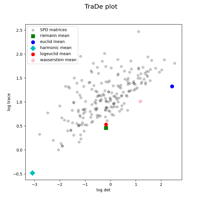
Means¶

TraDe plot displays the log-trace as a function of the log-determinant for different means.

This figure reproduces Fig 7 of reference [3].

rs = np.random.RandomState(17)
X, _ = make_gaussian_blobs(
    n_matrices=100, n_dim=3, class_sep=3.0, class_disp=2.0, random_state=rs,
)

fig, ax = plt.subplots(figsize=(7, 7))
fig.suptitle("TraDe plot", fontsize=16)
ax.set(xlabel="log det", ylabel="log trace")
ax.scatter(
    np.log10(np.linalg.det(X)),
    np.log10(np.trace(X, axis1=-2, axis2=-1)),
    c="k",
    alpha=0.2,
    label="SPD matrices"
)

metrics = ["riemann", "euclid", "harmonic", "logeuclid", "wasserstein"]
markers = ["s", "8", "D", "H", "h"]
colors = ["g", "b", "c", "r", "pink"]
for metric, marker, color in zip(metrics, markers, colors):
    M = gmean(X, metric=metric)
    ax.scatter(
        np.log10(np.linalg.det(M)),
        np.log10(np.trace(M)),
        c=color,
        marker=marker,
        s=80,
        label=metric + " mean"
    )
ax.legend()
plt.show()

References¶

Total running time of the script: (0 minutes 1.520 seconds)

Gallery generated by Sphinx-Gallery