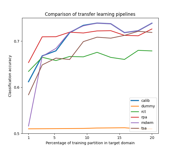
Comparison of pipelines for transfer learning

We compare the classification performance of MDM on five different strategies for transfer learning. These include re-centering the datasets as done in [1], matching the statistical distributions in a semi-supervised way with Riemannian Procrustes Analysis [2], and improving the MDM classifier with a weighting scheme (MDWM) [3]. All data points are simulated from a toy model based on the Riemannian Gaussian distribution and the differences in statistics between source and target distributions are determined by a set of parameters that have control over the distance between the centers of each dataset, the angle of rotation between the means of each class, and the differences in dispersion of the data points from each dataset.

from tqdm import tqdm

import numpy as np
import matplotlib.pyplot as plt
from sklearn.pipeline import make_pipeline
from sklearn.model_selection import StratifiedShuffleSplit

from pyriemann.classification import MDM
from pyriemann.datasets.simulated import make_classification_transfer
from pyriemann.transfer import (
    TLSplitter,
    TLDummy,
    TLCenter,
    TLStretch,
    TLRotate,
    TLClassifier,
    MDWM
)

Choose seed for reproducible results

seed = 100

# We consider several types of pipeline for transfer learning
# dummy : no transformation of dataset between the domains
# rct : re-center the data points from each domain to the Identity
# rpa : re-center, stretch and rotate (Riemannian Procrustes Analysis)
# mdwm : transfer learning with minimum distance to weighted mean
# calibration : use only data from target-train partition for the classifier
scores = {meth: [] for meth in ['dummy', 'rct', 'rpa', 'mdwm', 'calibration']}

# Create a dataset with two domains, each with two classes both datasets
# are generated by the same generative procedure with the SPD Gaussian
# and one of them is transformed by a matrix A, i.e. X <- A @ X @ A.T
X_enc, y_enc = make_classification_transfer(
    n_matrices=100,
    class_sep=0.75,
    class_disp=1.0,
    domain_sep=5.0,
    theta=3*np.pi/5,
    random_state=seed,
)

# Object for splitting the datasets into training and validation partitions
# the training set is composed of all data points from the source domain
# plus a partition of the target domain whose size we can control
target_domain = 'target_domain'
n_splits = 5  # how many times to split the target domain into train/test
tl_cv = TLSplitter(
    target_domain=target_domain,
    cv=StratifiedShuffleSplit(n_splits=n_splits, random_state=seed),
)

# Which base classifier to consider
clf_base = MDM()

# Vary the proportion of the target domain for training
target_train_frac_array = np.linspace(0.01, 0.20, 10)
for target_train_frac in tqdm(target_train_frac_array):

    # Change fraction of the target training partition
    tl_cv.cv.train_size = target_train_frac

    # Create dict for storing results of this particular CV split
    scores_cv = {meth: [] for meth in scores.keys()}

    # Carry out the cross-validation
    for train_idx, test_idx in tl_cv.split(X_enc, y_enc):

        # Split the dataset into training and testing
        X_enc_train, X_enc_test = X_enc[train_idx], X_enc[test_idx]
        y_enc_train, y_enc_test = y_enc[train_idx], y_enc[test_idx]

        # (1) Dummy pipeline: no transfer learning at all.
        # Classifier is trained only with samples from the source dataset.
        pipeline = make_pipeline(
            TLDummy(),
            TLClassifier(
                target_domain=target_domain,
                estimator=clf_base,
                domain_weight={'source_domain': 1.0, 'target_domain': 0.0},
            ),
        )

        # Fit and get accuracy score
        pipeline.fit(X_enc_train, y_enc_train)
        scores_cv['dummy'].append(pipeline.score(X_enc_test, y_enc_test))

        # (2) RCT pipeline: recenter data from each domain to identity [1]_.
        # Classifier is trained only with points from the source domain.
        pipeline = make_pipeline(
            TLCenter(target_domain=target_domain),
            TLClassifier(
                target_domain=target_domain,
                estimator=clf_base,
                domain_weight={'source_domain': 1.0, 'target_domain': 0.0},
            ),
        )

        pipeline.fit(X_enc_train, y_enc_train)
        scores_cv['rct'].append(pipeline.score(X_enc_test, y_enc_test))

        # (3) RPA pipeline: recenter, stretch, and rotate [2]_.
        # Classifier is trained with points from source and target.
        pipeline = make_pipeline(
            TLCenter(target_domain=target_domain),
            TLStretch(
                target_domain=target_domain,
                final_dispersion=1,
                centered_data=True,
            ),
            TLRotate(target_domain=target_domain, metric='euclid'),
            TLClassifier(
                target_domain=target_domain,
                estimator=clf_base,
                domain_weight={'source_domain': 0.5, 'target_domain': 0.5},
            ),
        )

        pipeline.fit(X_enc_train, y_enc_train)
        scores_cv['rpa'].append(pipeline.score(X_enc_test, y_enc_test))

        # (4) MDWM pipeline
        domain_tradeoff = 1 - np.exp(-25*target_train_frac)
        pipeline = MDWM(domain_tradeoff=domain_tradeoff,
                        target_domain=target_domain)
        pipeline.fit(X_enc_train, y_enc_train)
        scores_cv['mdwm'].append(pipeline.score(X_enc_test, y_enc_test))

        # (5) Calibration: use only data from target-train partition.
        # Classifier is trained only with points from the target domain.
        pipeline = make_pipeline(
            TLClassifier(
                target_domain=target_domain,
                estimator=clf_base,
                domain_weight={'source_domain': 0.0, 'target_domain': 1.0},
            ),
        )

        pipeline.fit(X_enc_train, y_enc_train)
        scores_cv['calibration'].append(pipeline.score(X_enc_test, y_enc_test))

    # Get the average score of each pipeline
    for meth in scores.keys():
        scores[meth].append(np.mean(scores_cv[meth]))

# Store the results for each method on this particular seed
for meth in scores.keys():
    scores[meth] = np.array(scores[meth])

  0%|          | 0/10 [00:00<?, ?it/s]
 10%|█         | 1/10 [00:00<00:05,  1.50it/s]
 20%|██        | 2/10 [00:01<00:06,  1.33it/s]
 30%|███       | 3/10 [00:02<00:05,  1.29it/s]
 40%|████      | 4/10 [00:03<00:04,  1.30it/s]
 50%|█████     | 5/10 [00:03<00:03,  1.33it/s]
 60%|██████    | 6/10 [00:04<00:02,  1.35it/s]
 70%|███████   | 7/10 [00:05<00:02,  1.37it/s]
 80%|████████  | 8/10 [00:05<00:01,  1.41it/s]
 90%|█████████ | 9/10 [00:06<00:00,  1.41it/s]
100%|██████████| 10/10 [00:07<00:00,  1.40it/s]
100%|██████████| 10/10 [00:07<00:00,  1.37it/s]

Plot the results, reproducing Figure 2 of [2].

fig, ax = plt.subplots(figsize=(6.7, 5.7))
for meth in scores.keys():
    ax.plot(
        target_train_frac_array,
        scores[meth],
        label=meth,
        lw=3.0)
ax.legend(loc='lower right')
ax.set_ylim(0.45, 0.75)
ax.set_yticks([0.5, 0.6, 0.7])
ax.set_xlim(0.00, 0.21)
ax.set_xticks([0.01, 0.05, 0.10, 0.15, 0.20])
ax.set_xticklabels([1, 5, 10, 15, 20])
ax.set_xlabel('Percentage of training partition in target domain')
ax.set_ylabel('Classification accuracy')
ax.set_title('Comparison of transfer learning pipelines')

plt.show()

References

[1]

Transfer Learning: A Riemannian Geometry Framework With Applications to Brain–Computer Interfaces P Zanini et al, IEEE Transactions on Biomedical Engineering, vol. 65, no. 5, pp. 1107-1116, August, 2017

[2] (1,2)

Riemannian Procrustes analysis: transfer learning for brain-computer interfaces PLC Rodrigues et al, IEEE Transactions on Biomedical Engineering, vol. 66, no. 8, pp. 2390-2401, December, 2018

[3]

Transfer Learning for SSVEP-based BCI using Riemannian similarities between users E Kalunga et al, 26th European Signal Processing Conference (EUSIPCO 2018) Sep 2018, Rome, Italy, pp.1685-1689